How categorical Jacobians retrieve contact maps

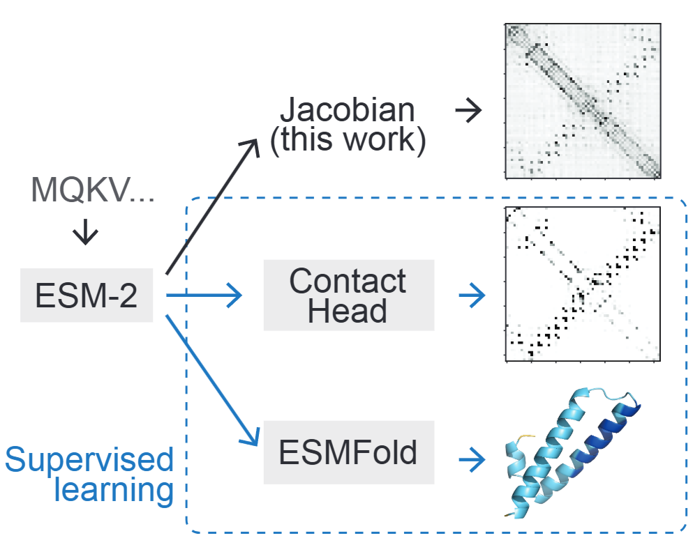
A protein’s structure is completely determined by the sequence of amino acids making it up. This suggests that protein language models, trained on billions of protein sequences, can be leveraged to predict protein structure. And certainly that’s true: if you do supervised training on ESM-2 embeddings, you get ESMFold, which rivals AlphaFold2 in accuracy while running faster and not requiring sequence alignment data. But the supervised approach requires gathering millions of real and AlphaFold-predicted structures.

A creative 2024 paper from Sergey Ovchinnikov’s group produces structure contact maps in a completely unsupervised way, using a method they call the “categorical Jacobian”. Unfortunately, their paper isn’t the easiest to follow. In this post, I aim to explain categorical Jacobians clearly. Even if you don’t care about protein structure prediction, this should be a fun machine learning case study: the authors really thought hard about using an LLM’s internal representations for a novel task.

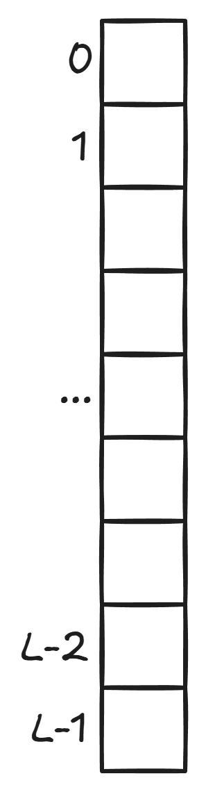
Imagine a protein made up of $L$ amino acids as this sequence:

A key question categorical Jacobians ask is: if you change the amino acid at position $p$, how much do the model’s predictions for the amino acid at position $q$ change?

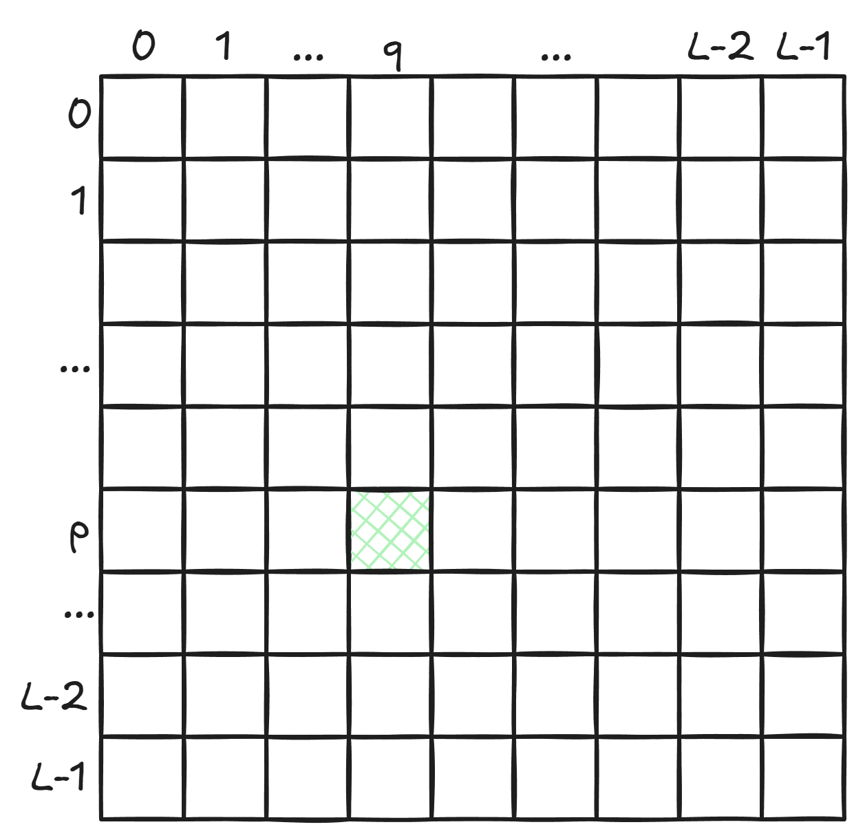
If the model’s predictions for position $q$ depend a lot on what’s at position $p$, it suggests that the amino acids co-occur frequently enough in the training data for the model to memorize. The model then uses this memorized information and what it knows about the amino acid at position $p$ to make predictions at position $q$.

Now, why might two amino acids co-occur? Often because they’re in contact with each other.¹ If they were not, one of the amino acids could mutate into something else, while the other stayed the same, without destabilizing the protein. The mutation would spread through the gene pool because it’s harmless, weakening the co-occurring signal. But if the amino acids are in contact, and one of them mutates into an amino acid with different chemical properties, the contact would break, likely destabilizing the protein. The protein was presumably important (otherwise, natural selection wouldn’t let the organism waste resources expressing it). The organism with the malformed protein would be disadvantaged, and the mutation wouldn’t spread through the gene pool. Thus, the amino acid co-occurrence in the training data would remain strong. Liam Bai dives deeper into this intuition in this blog post. This section of the blog post “Can We Learn the Language of Proteins?” is also great.

This notion of “how sensitive the prediction at $q$ is to the amino acid at $p$” can be captured by a $20 \times 20$ matrix for each cell of the $L \times L$ matrix.

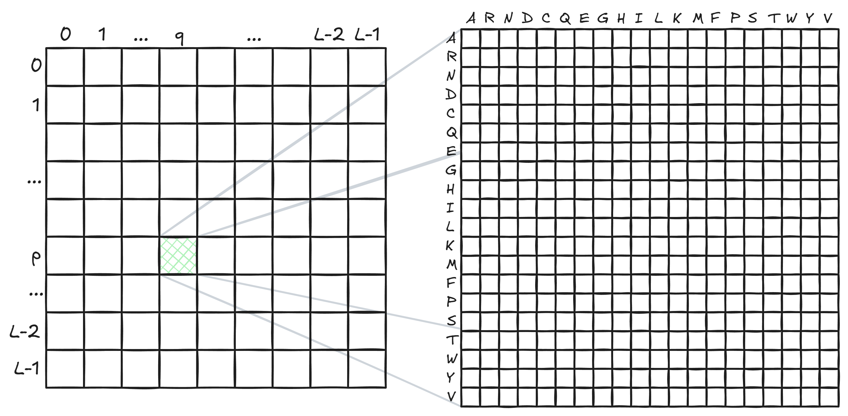
Here is how every cell of the amino acid grid is filled: to fill the first row, mutate the token at position $p$ to the amino acid $A$ (alanine). Given this mutation, how much does the logit for amino acid $A$ at position $q$ change? Say it goes up by $+1.02$. That’s the first column of the first row (i.e., cell $(A, A)$). How much does the logit for amino acid $R$ (arginine) at position $q$ change? Say it changes by $-0.84$ (i.e., it goes down, meaning that $q$ being $R$ becomes less likely). That’s the second column of the first row (i.e., cell $(A, R)$). Repeat for all possible amino acids at position $q$ (all columns), then repeat for all possible mutations at position $p$ (all rows).

So, in the completed amino acid grid, position $(Q, D)$, for example, would answer the question: if position $p$ were the amino acid $Q$ (glutamine), by how much would the logit for the amino acid $D$ (aspartic acid) at position $q$ change?

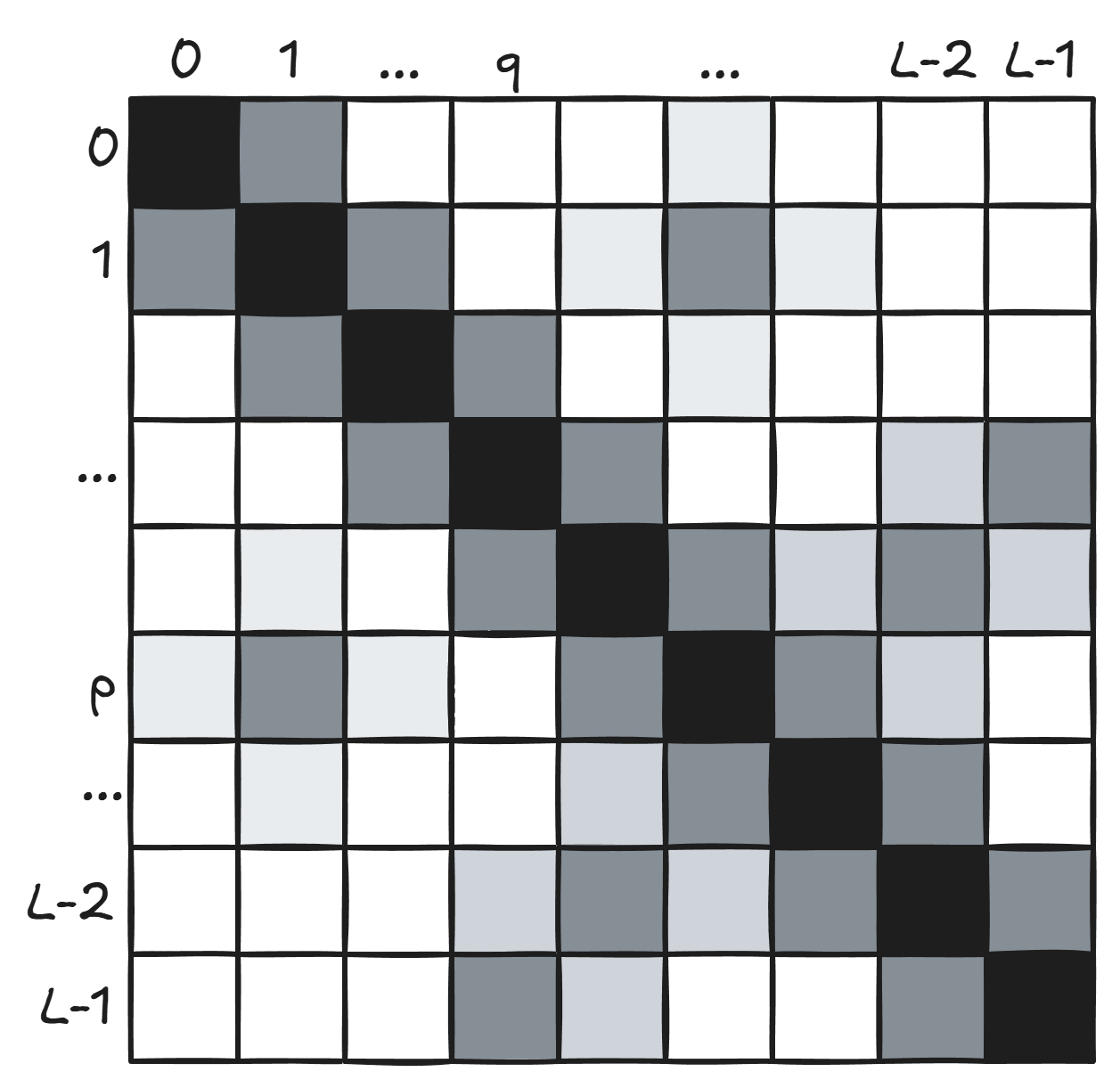
If you take the Frobenius norm (root mean square) of every value in the amino acid grid, you get a single number that tells you how much position $p$ co-varies with position $q$. Plop this single number into position $(p, q)$ in the $L \times L$ grid. Repeat for every cell in the $L \times L$ grid.

The resulting $L \times L$ matrix is a “covariation map” (and, because of the co-occurrence logic I described above, effectively a contact map):

This figure from the paper shows how close the covariation map looks to a contact map predicted using supervised learning from ESM-2 embeddings:

Here’s a rudimentary PyTorch implementation of the categorical Jacobian (absent mean-centering, symmetrization, and a denoising step called average product correction, which I won’t get into in this blog post):

import torch

L = len(sequence)
A = 20  # amino acid alphabet size

# Get original logits [L, A]
original_logits = model(sequence.unsqueeze(0)).squeeze(0)

# Initialize Jacobian [L, A, L, A]
jacobian = torch.zeros(L, A, L, A)

# For each position and amino acid mutation
for p in range(L):
    for a in range(A):
        # Mutate position p to amino acid a
        mutated_seq = sequence.clone()
        mutated_seq[p] = a

        # Get difference in logits
        mutated_logits = model(mutated_seq.unsqueeze(0)).squeeze(0)
        jacobian[p, a, :, :] = mutated_logits - original_logits

# Extract L x L contact map from jacobian [L, A, L, A]
covariation_map = torch.norm(jacobian, dim=(1, 3))  # norm over A x A dimensions

# covariation_map[p, q] = covariation strength between positions p and q

Categorical Jacobians work in a number of biology sequence models beyond ESM-2, which was studied in the Ovchinnikov paper. For example, Tatta Bio’s 650M-parameter model gLM2 was able to find inter-protein contacts in the ModABC transporter complex with categorical Jacobians, and in his podcast with Abhishaike Mahajan, Sergey Ovchinnikov says that categorical Jacobians with the autoregressive DNA language model Evo 2 pinpoint RNA interactions.