Allreduce (and the rest) from scratch
A distributed training run is a stack of matrix multiplies separated by a small number of communication patterns. Those patterns are the collectives: allreduce, allgather, reduce-scatter, broadcast, all-to-all. Every modern parallelism strategy is a particular sequence of these.
Every collective, in turn, is a schedule of exactly two primitives: a
point-to-point send and a point-to-point recv. To make this concrete, I
handrolled each of them from PyTorch’s
dist.send/dist.recv.
The code (implementations, tests, and benchmark) is in this GitHub repo.
This post walks through each collective with a steppable animation.
Understanding each lets you model data parallelism (DDP) as an allreduce
on the gradients, ZeRO / FSDP as a
reduce_scatter on gradients plus an allgather on parameters, tensor
parallelism as an allreduce (or allgather/reduce_scatter) on
activations, and mixture of experts
(MoE) routing as an all_to_all.
This leads to some counterintuitive facts becoming obvious: e.g., why ZeRO-2 buys a large memory saving for zero extra communication over DDP, and why deep learning communication libraries almost always pick ring scheduling over tree.
The alpha-beta cost model
Sending a message of $M$ bytes from one rank to another costs
\[T_{\text{p2p}} = \alpha + \beta M.\]$\alpha$ is the fixed per-message latency (the handshake, the kernel crossing, etc.) and $\beta$ is the per-byte cost (the reciprocal of bandwidth). This is the Hockney model. While crude — it ignores congestion and topology — it’s powerful enough for our purposes.
A collective’s wall time is
\[T = (\text{messages on the critical path}) \cdot \alpha + (\text{bytes on the busiest link}) \cdot \beta.\]So every algorithm earns two numbers: a coefficient on $\alpha$ (how many sequential message rounds it takes) and a coefficient on $\beta M$ (how many $M$-sized payloads cross the bottleneck link). With $N$ ranks and a total message of size $M$, here is the scorecard for everything in this post:
| collective | pattern | $\alpha$ coef | $\beta M$ coef | notes |
|---|---|---|---|---|
broadcast_flat |
flat from root | $N-1$ | $N-1$ | baseline |
broadcast_tree |
binomial tree | $\log N$ | $\log N$ | latency-optimal |
scatter |
flat from root | $N-1$ | $(N-1)/N$ | |
gather |
flat to root | $N-1$ | $(N-1)/N$ | |
reduce_flat |
flat to root | $N-1$ | $N-1$ | baseline |
reduce_tree |
binomial tree | $\log N$ | $\log N$ | latency-optimal |
allgather |
ring | $N-1$ | $(N-1)/N$ | bandwidth-optimal |
reduce_scatter |
ring | $N-1$ | $(N-1)/N$ | bandwidth-optimal |
allreduce_ring |
RS + AG | $2(N-1)$ | $2(N-1)/N$ | bandwidth-optimal |
allreduce_tree |
reduce + bcast | $2\log N$ | $2\log N$ | latency-optimal |
all_to_all |
pairwise | $N-1$ | $(N-1)/N$ | bandwidth-optimal |
There are two ways an algorithm could be efficient. It could minimize rounds — get the $\alpha$ coefficient down. Or it could minimize bytes per link — bring the $\beta M$ coefficient down. Rounds are minimized with trees, and bytes per link are minimized with rings. Rings win when $M$ is large, so the $\beta M$ term dominates (bandwidth-bound); trees win when $M$ is small, so the $\alpha$ term dominates (latency-bound).
Rooted collectives
The simplest way to move data is to put one rank in charge. These four collectives all have a root that talks to everyone else in a star.
broadcast_flat
The root holds the data and sends a copy to each of the $N-1$ other ranks, one message at a time. The root’s link is the bottleneck: $N-1$ sequential messages, each carrying the full $M$ bytes. This is the baseline we’ll beat later with a tree.
def broadcast_flat(rank, world_size, data, root=0):
    if rank == root:
        for peer in range(world_size):
            if peer != root:
                dist.send(data, dst=peer)
    else:
        dist.recv(data, src=root)
scatter
The root holds $N$ chunks and sends chunk $i$ to rank $i$ — like a broadcast, except each peer receives a different $M/N$ slice rather than the whole thing. Still $N-1$ sequential sends from the root, but only $M/N$ bytes each, so the $\beta M$ coefficient drops to $(N-1)/N$. $(N-1)/N$ tends to $1$ as network size increases.
def scatter(rank, world_size, data, root=0):
    # Require data size divisibility by world size. Otherwise, chunks may have
    # uneven lengths, and we'd need either two sendrecvs instead of one (one
    # for chunk size to allocate an appropriately-sized buffer, and one for the raw
    # data itself) or padding.
    assert data.numel() % world_size == 0, "data size must be divisible by world_size"
    chunk_size = data.numel() // world_size
    if rank == root:
        chunks = data.chunk(world_size)
        for peer in range(world_size):
            if peer != root:
                dist.send(chunks[peer], dst=peer)
        return chunks[root].clone()
    else:
        buf = torch.empty(chunk_size, dtype=data.dtype)
        dist.recv(buf, src=root)
        return buf
gather
The exact inverse of scatter: every rank sends its $M/N$ chunk to the root, which concatenates them in rank order.
def gather(rank, world_size, data, root=0):
    if rank == root:
        chunks = [torch.empty_like(data) for _ in range(world_size)]
        chunks[root] = data
        for peer in range(world_size):
            if peer != root:
                dist.recv(chunks[peer], src=peer)
        return torch.cat(chunks)
    else:
        dist.send(data, dst=root)
        return None
reduce_flat
Like gather, but the root sums the incoming tensors instead of concatenating
them. Each peer sends its full $M$ bytes and the root accumulates. So, unlike
gather, the $\beta M$ coefficient is $N-1$, not $(N-1)/N$. This is another
baseline a tree implementation beats.
def reduce_flat(rank, world_size, data, root=0):
    if rank == root:
        result = data.clone()
        buf = torch.empty_like(data)
        for peer in range(world_size):
            if peer != root:
                dist.recv(buf, src=peer)
                result += buf
        return result
    else:
        dist.send(data, dst=root)
        return None
The pattern across all four is that the root performs $N-1$ messages back to
back, so latency scales as $N-1$. scatter and gather move only $M/N$ per
message; broadcast and reduce move a full $M$. A tree fixes the serial root:
it lets children which have received the data to start propagating it.
The binomial tree
Having the root do all $N-1$ messages sequentially idles NIC capacity at the other ranks. A tree parallelizes the work. At every round, each rank that’s already received the data passes it on. The number of holders doubles each round, so after $\lceil \log_2 N \rceil$ rounds every rank has it.
For broadcast_tree with $N = 8$, rank 0 sends to rank 4; then 0 and 4 each
seed a partner two away (0 to 2, 4 to 6); then those four each seed a partner
one away (0 to 1, 2 to 3, 4 to 5, 6 to 7). reduce_tree is the mirror image, in
which the active set halves each round as partial sums fold inward toward 0. The
neat implementation trick is that a rank’s lowest set bit tells it which round
it joins in, so the schedule is bit twiddling.
broadcast_tree
def broadcast_tree(rank, world_size, data):
    n_rounds = (world_size - 1).bit_length()
    for k in range(n_rounds - 1, -1, -1):
        distance = 1 << k
        # A rank's lowest set bit is its round of arrival -- the round where it
        # receives the data and joins the holder set. Once it arrives, it
        # remains active for all rounds with smaller k, where it serves as a
        # sender to grow its own subtree.
        # This check: if any lower bit set, rank doesn't receive data yet; skip
        # for a later (smaller-k) round.
        if rank & (distance - 1):
            continue
        # If rank's lowest set bit is k, receive and join the holder set.
        if rank & distance:
            dist.recv(data, src=rank - distance)
        # Data flows from bit-k-clear rank to its bit-k-set peer at rank + 2^k.
        else:
            peer = rank + distance
            if peer < world_size:
                dist.send(data, dst=peer)
reduce_tree
def reduce_tree(rank, world_size, data):
    acc = data.clone()
    buf = torch.empty_like(data)
    n_rounds = (world_size - 1).bit_length()
    for k in range(n_rounds):
        # 1 << k = 2^k. At round 0 you pair with your distance-1 neighbor, round
        # 1 with distance-2, round 2 with distance-4, etc.
        distance = 1 << k
        # Rank with k-th bit set sends.
        if rank & distance:
            # Send our running sum to the peer, then drop out.
            dist.send(acc, dst=rank - distance)
            return None
        peer = rank + distance
        if peer < world_size:
            dist.recv(buf, src=peer)
            acc += buf
    # Rank 0 has all bits zero, so it never enters the send branch and is the
    # only rank to reach this return with the full sum.
    return acc
The payoff is going from $N-1$ rounds to just $\lceil \log_2 N \rceil$ rounds. For $N = 8$ that is seven down to three. But notice that every round still ships a full $M$-byte message on the active links, so the total bytes moved across the critical path grow as $M \log N$. A bandwidth fix lies in noticing a lower bound on the per-link payload, and slashes the $\beta M$ coefficient down to a constant.
The ring
The ring’s observation is that you need never move more than $M/N$ bytes at a time.
allgather
Every rank starts with one chunk, and every rank must end up with all $N$ chunks. Imagine the ranks arranged in a circle. On each step, every rank sends the chunk it currently holds to its right neighbor and receives a new chunk from its left. After $N-1$ steps, every chunk has visited every rank.
Before the code for the schedule, an implementation detail: ordering. gloo’s
send blocks once the payload outgrows the kernel’s socket buffer. So if every
rank runs the symmetric “send to my partner, then receive from my partner”,
every rank blocks in send waiting for a matching recv.
To break the symmetry, we need a deterministic rule both sides can compute independently. The simplest is “even ranks send first / odd ranks receive first” (we’ll use its cousin, “lower rank sends first”, for all-to-all later).
def allgather(rank, world_size, data):
    left = (rank - 1) % world_size
    right = (rank + 1) % world_size

    chunks = [torch.empty_like(data) for _ in range(world_size)]
    chunks[rank] = data.clone()

    send_idx = rank
    for _ in range(world_size - 1):
        recv_idx = (send_idx - 1) % world_size
        # Even ranks send first, odd ranks recv first
        if rank % 2 == 0:
            dist.send(chunks[send_idx], dst=right)
            dist.recv(chunks[recv_idx], src=left)
        else:
            dist.recv(chunks[recv_idx], src=left)
            dist.send(chunks[send_idx], dst=right)
        send_idx = recv_idx

    return torch.cat(chunks)
Each step moves only $M/N$ bytes per link, over $N-1$ steps, for a total of $M(N-1)/N$ bytes per link. This is bandwidth-optimal. To end up holding everyone else’s data, each rank must receive at least $M(N-1)/N$ bytes (every chunk but its own), and the ring hits that lower bound exactly. You cannot move fewer bytes. The price is latency: $N-1$ sequential steps, the same as the flat version.
reduce_scatter
The mirror of allgather. Now every rank starts with the full $M$ (all $N$ chunks) and we want rank $r$ to end with the sum across all ranks of chunk $r$. Same ring rotation, except the receiver adds the incoming chunk into its local copy instead of overwriting. After $N-1$ steps, rank $r$ holds the fully reduced chunk $r$.
def reduce_scatter(rank, world_size, data):
    assert data.numel() % world_size == 0, "data size must be divisible by world_size"
    left = (rank - 1) % world_size
    right = (rank + 1) % world_size

    chunks = [chunk.clone() for chunk in data.chunk(world_size)]
    buf = torch.empty_like(chunks[0])

    send_idx = (rank - 1) % world_size
    for _ in range(world_size - 1):
        recv_idx = (send_idx - 1) % world_size
        if rank % 2 == 0:
            dist.send(chunks[send_idx], dst=right)
            dist.recv(buf, src=left)
        else:
            dist.recv(buf, src=left)
            dist.send(chunks[send_idx], dst=right)
        chunks[recv_idx] += buf
        send_idx = recv_idx

    return chunks[rank]
Allreduce, and why ZeRO-2 is free
Allreduce leaves every rank holding the elementwise sum of every rank’s input. It’s the workhorse of data-parallel training: each rank computes gradients on its slice of the batch, and an allreduce averages them so every rank can take the same optimizer step. There are two natural implementations.
allreduce_ring
A reduce-scatter followed by an allgather. After the reduce-scatter, rank $r$ owns the fully summed chunk $r$. An allgather then hands those summed chunks to everyone. That is the actual implementation:
def allreduce_ring(rank, world_size, data):
    reduced_chunk = reduce_scatter(rank, world_size, data)
    return allgather(rank, world_size, reduced_chunk)
The cost is $2(N-1)$ on $\alpha$ and $2(N-1)/N$ on $\beta M$ — bandwidth-optimal, the factor of two being the unavoidable cost of getting data out and back.
allreduce_tree
A reduce followed by a broadcast. Fold everything to rank 0 with reduce_tree,
then broadcast_tree the result back out. Cost $2\log N$ on both coefficients
— latency-optimal.
def allreduce_tree(rank, world_size, data):
    reduced = reduce_tree(rank, world_size, data)
    out = reduced if rank == 0 else torch.empty_like(data)
    broadcast_tree(rank, world_size, out)
    return out
The identity allreduce = reduce-scatter + allgather explains the free lunch
that powers ZeRO-2. In plain data parallel (DDP), every rank stores a full copy
of the parameters, the gradients, and the optimizer states. For Adam in mixed
precision, the optimizer states (fp32 master weights, momentum, variance) come
to roughly three times the size of the parameters themselves. So, across $N$
ranks, you store $N$ identical copies of the weightiest tensor in the system.
Each step: compute local gradients, allreduce them, and every rank runs the
identical optimizer update on the full parameter set.
ZeRO (the Zero Redundancy Optimizer underlying DeepSpeed, and the idea behind PyTorch FSDP) shards this redundancy away. ZeRO-1 shards the optimizer states; ZeRO-2 additionally shards the gradients; ZeRO-3 additionally shards the parameters. Specifically, ZeRO-2, instead of an allreduce on the gradients, does:
reduce_scatterthe gradients, so rank $r$ ends up holding the summed gradient for only its shard $r$;- rank $r$ updates only its shard of the parameters, using only its shard of the optimizer states;
allgatherthe updated parameter shards, so every rank has the full parameters again for the next forward pass.
If you count the bytes, DDP does one allreduce on the gradients, which is a reduce-scatter plus an allgather under the hood. ZeRO-2 does one reduce-scatter on the gradients plus one allgather on the parameters. Parameters and gradients are the same size, so ZeRO-2 moves exactly the same number of bytes as DDP. You get an $N$-fold reduction in gradient and optimizer-state memory for zero additional communication.
(The free lunch ends at ZeRO-3. Sharding the parameters means they have to be
allgather-ed back in both the forward and the backward pass, which pushes
total communication to roughly 1.5x. ZeRO-3 trades communication for the ability
to fit the model at all.)
Why deep learning picks the ring over the tree
For an allreduce, which algorithm should you pick: ring or tree? Plug $N = 8$ into the scorecard: the ring has $2(8-1) = 14$ rounds of latency, and $2(8-1)/8 = 1.75$ payloads of bandwidth; the tree has $2\log_2 8 = 6$ rounds of latency, and $2\log_2 8 = 6$ payloads of bandwidth.
The tree does fewer rounds (6 versus 14) but moves far more bytes (6 versus
1.75). So the tree wins when $\alpha$ dominates (small messages) and the ring
wins when $\beta M$ dominates (large messages). To reproduce the crossover for
myself, I benchmarked both handrolled allreduces against gloo’s built-in
dist.all_reduce on 8 CPU ranks, sweeping message size. Log-scaled-y and
linear-scaled-y views:
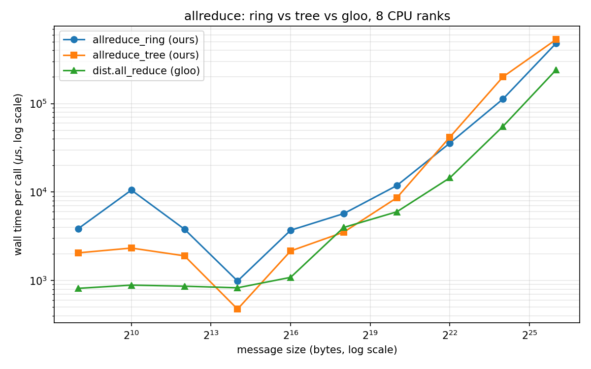
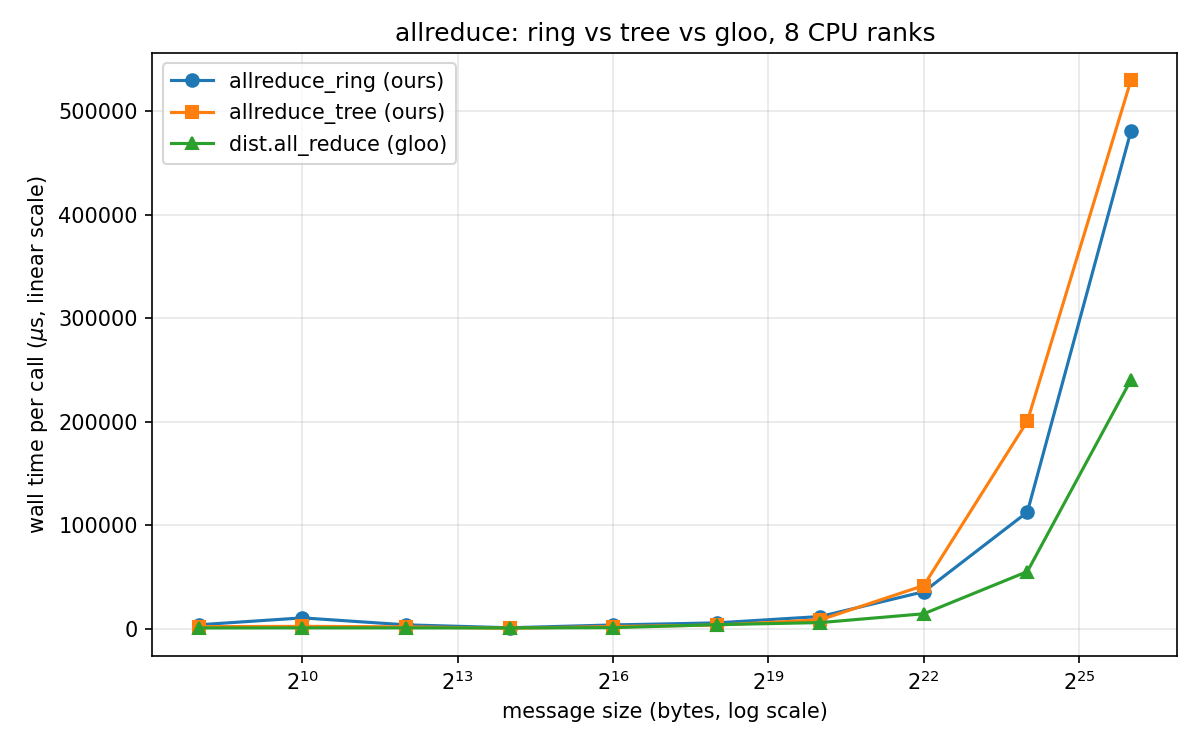
Tree leads through 1 MB, the curves cross somewhere between 1 and 4 MB, and ring wins from 4 MB up (at 64 MB, ring averages about 0.48 s against tree’s 0.53 s). (On NCCL, the crossover point lands in the same order of magnitude.) Expectedly, gloo’s C implementation beats both of my Python-loop versions almost everywhere — orchestrating sends and receives from a Python loop incurs overhead.
The deep learning punchline: gradient buffers are big. A 7-billion-parameter model in bf16 has a 14 GB gradient tensor. Even though DDP buckets the gradients, firing allreduce on every ~25 MB bucket as it fills to overlap communication with the backward pass, a single bucket is already one to two orders of magnitude past the crossover. Deep learning is firmly bandwidth-bound.
This is why, though NCCL keeps a tree algorithm (a clever double binary tree) around for the small-message, latency-bound regime, for averaging gradients it’s rings; the tree’s $\log N$ latency edge matters little when every message is MBs to GBs.
All-to-all, the MoE collective
all_to_all
The final collective is the most symmetric of all: all_to_all is a matrix
transpose. Each rank holds $N$ chunks, and chunk $j$ on rank $i$ goes to rank
$j$.
This is bandwidth-optimal, at $(N-1)/N$ on $\beta M$. The subtlety is scheduling: if every rank walks its partners in the same order $0, 1, 2, \dots$, they all pile onto the same partner each step and the round serializes as gloo’s sends block, waiting for a matching recv. Pairing instead by $\text{peer} = \text{rank} \oplus k$ for $k = 1, \dots, N-1$ (when $N$ is a power of two) keeps every rank busy with a distinct partner on every step, so the rounds run in parallel.
Why does XOR give that clean matching? For any fixed $k$, the map $\text{rank} \mapsto \text{rank} \oplus k$ is its own inverse and has no fixed point (XOR by something nonzero must change at least one bit), so it splits all $N$ ranks into $N/2$ mutual pairs — one conflict-free round. And the pair ${a, b}$ is hit by exactly one mask, $k = a \oplus b$, so the $N-1$ rounds together pair every rank with every other one exactly once.
This random-looking butterfly pattern makes much more sense if you visualize it in a higher dimension. With $N = 2^d$ ranks, every rank is a corner of a $d$-dimensional hypercube. Two corners share an edge exactly when their labels differ in a single bit. This is a poor man’s coordinate system: XOR-ing a rank by $k$ flips exactly the bits set in $k$, so $\text{rank} \oplus k$ is the corner you reach by stepping along every axis named in $k$ at once. The animation below puts the 8 ranks on a cube and steps through the masks.
def all_to_all(rank, world_size, data):
    assert data.numel() % world_size == 0, "data size must be divisible by world_size"
    chunks = list(data.chunk(world_size))
    # Diagonal of the transpose: my own j=rank chunk stays put.
    out = [torch.empty_like(chunks[0]) for _ in range(world_size)]
    out[rank] = chunks[rank].clone()
    ws_is_pow2 = world_size & (world_size - 1) == 0
    for k in range(1, world_size):
        # XOR schedule when N is a power of 2, otherwise the plain linear peer
        # order. XOR-by-k is a fixed-point-free (nobody is paired with
        # themselves) involution (applying it twice gets you back where you
        # started, so the pairing is mutual -- both sides are partners this
        # step). This results in a "perfect matching": every node is paired with
        # exactly one other node, and no node appears in two pairs, i.e., every
        # step cleanly splits all N ranks into N/2 disjoint pairs.
        #
        # In linear peer order, you get a star centered on a single hub instead
        # of a matching, resulting in serialization.
        peer = rank ^ k if ws_is_pow2 else k
        # This guard fires only on the non-pow2 branch since XOR-by-k is
        # fixed-point-free.
        if peer == rank:
            continue
        # Lower rank sends first to break the symmetry.
        if rank < peer:
            dist.send(chunks[peer], dst=peer)
            dist.recv(out[peer], src=peer)
        else:
            dist.recv(out[peer], src=peer)
            dist.send(chunks[peer], dst=peer)
    return torch.cat(out)
A transpose-shaped communication pattern shows up most canonically in deep
learning in MoE layers. Experts are sharded across ranks, and a router sends
each token to a few of them. So, after routing, every rank holds a pile of
tokens destined for experts that live on other ranks. Dispatching the tokens to
the right experts is an all_to_all, and gathering the experts’ outputs back to
the tokens’ home ranks is another. MoE training and inference are often
all-to-all-bound, which explains the effort poured into interconnect bandwidth
and expert placement.
The code
The full implementations, tests, and benchmark are on GitHub.