Fresnel, Perlin, bloom, and other ways to fake realism in graphics
Graphics programmers have invented a host of tricks to cheaply bring realism to a scene. This post goes through some of the greatest hits: scripted sequences, Fresnel, specular glint, Perlin noise, billboarding, etc. It is my final project for Northwestern’s CS 351: Intro to Computer Graphics.
The scene’s core loop is a dragon circling, diving, and taking off. It’s something of a system: butterflies scatter when the dragon lands, and the tree canopy sways from the wingbeats. The sun and the moon traverse a day/night cycle, the light is redder during dawn and dusk, and stars appear in the night. The terrain is procedurally generated from noise, and the hills are colored by elevation (tan peaks and grassy lows). The snake slithers forward/backward and climbs the tree if you hold Q/E. The pond has procedural ripples and effects like Fresnel reflections and specular glint. Bloom imparts a soft glow from the sun, the moon, and their reflections off of water, windmill metal, and dragon.
Instructions
Click the scene to activate interactions. Then, use mouse to look around (Esc releases it).
Space toggles camera modes:
- Free-flying:
WASDmove,R/Fup/down, arrow keys also look around. - Orbit:
W/Sin/out,A/Daround,R/Fraise/lower.
Q/E slither the python forward/backward. It climbs the tree when near the trunk.
Holding Shift fast-forwards the scene at 3x speed.
Credits
- WebGL and matrix helpers from course
cuonlibs. - 3D models and textures from Kim Whitney’s CS 351 collection.
- Perlin-noise implementation from course
terrain.jsby Evan Bertis-Sample and Prof. Dietrich Geisler.
Technical report
Source code is deliberately not shared per course instructions. Instead, I describe the key ideas in prose and snippets. You don’t really need a graphics background to understand these ideas; the prose should make sense to anyone who has some programming experience, and the snippets should read like pseudocode.
Water
Fresnel reflection
Fresnel is a slightly obscure physical effect that contributes a vast amount to what makes water reflect like water. It’s one of the most realism-per-line-of-shader-code effects in the project.
A straight-up 100% reflective pool looks like a wavy silvered mirror:
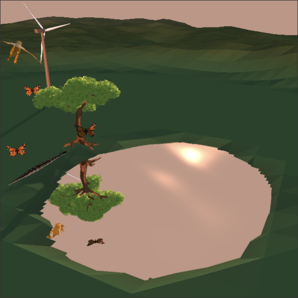
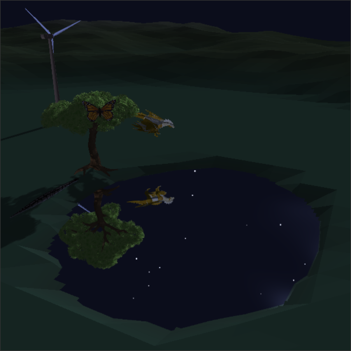
With Fresnel, you get water:
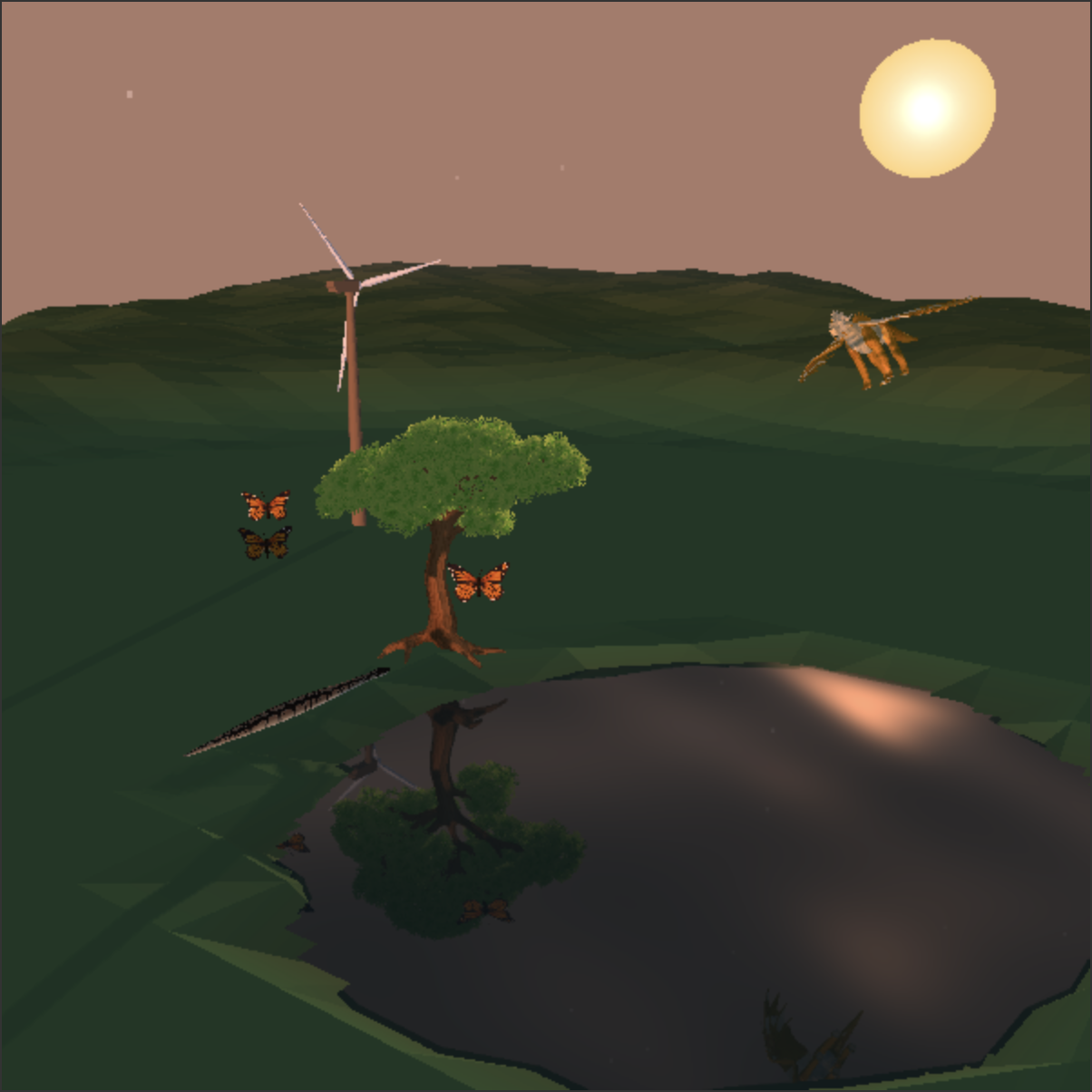
The physical intuition for Fresnel is that at a grazing angle, light travels almost parallel to the surface of water, so very little of its energy propagates in. At 89 degrees to the normal, 90% of light energy is reflected back, and only about a tenth refracts in. But from directly overhead, just 2% is reflected back. This is why a lake viewed from above can appear transparent or dark, while the distant surface near the horizon strongly reflects the sky.
First, a simple reflection is constructed:
x_refl = x
y_refl = 2h - y
z_refl = z
Ripples are procedural — three sine waves h(x,z,t) = A sin(k dot [x,z] + speed*t) because just one would look too mechanical.
The shader doesn’t actually compute the wave height, only its tangent plane, using the gradient:
vec2 rippleGrad(vec2 p, float t) {
    vec2 g = vec2(0.0);

    vec2 k1 = vec2(0.9, 0.6) * 1.7;
    g += 0.030 * cos(dot(p, k1) + t * 1.3) * k1;

    vec2 k2 = vec2(-0.6, 1.0) * 2.6;
    g += 0.018 * cos(dot(p, k2) + t * 1.7) * k2;

    vec2 k3 = vec2(0.4, -0.9) * 3.9;
    g += 0.010 * cos(dot(p, k3) + t * 2.3) * k3;

    return g;
}
The surface tangent vectors are Tz = [0, dh/dz, 1] and Tx = [1, dh/dx, 0]; their cross product gives the normal N = [-dh/dx, 1, -dh/dz]:
vec3 N = normalize(vec3(-grad.x, 1.0, -grad.y));
We dot(V, N) with the ripple normal so that 1 is looking downward, and 0 is along the surface. We use a Fresnel approximation with a hand-tuned cubic power and 10% reflection floor:
float fresnel_factor = mix(0.10, 1.0, pow(
    1.0 - max(dot(V, N), 0.0),
    3.0
));
// shader mixes the water body's dark blue tint with the scene reflection
vec3 col = mix(body, reflColor, fresnel_factor);
Specular glint
We also add “light glint” — a Blinn-Phong highlight which ripple normals break into moving streaks:
// halfway vector between the viewing and light directions
vec3 H = normalize(V + normalize(u_LightDir));
// exponent of 140 for narrow and bright
float spec = pow(max(dot(N, H), 0.0), 140.0);
// highlight uses the current key light color, so the sun creates a warm glint
// during the day and the moon creates a cool glint at night
col += u_LightColor * spec;
Specular light is the direct reflection of a light source (here, the sun and the moon). So, it makes sense that it’s most intense when you (the camera) are at an angle with the normal exactly equal to that the light source makes with the normal, and becomes sharply less intense as you deviate. dot(normal, halfway_vec_between_you_and_the_light_source) as the core input to the intensity spec is meant to capture precisely this intuition.
How to land your dragon
Locate the dragon
The world’s interactions with the dragon (butterflies fleeing, canopy swaying) use no physics. The dragon moves on a schedule, so the rest of the world can move on the same schedule.
Specifically, the dragon’s full landing cycle has a total duration of const DRAGON_CYCLE = 20000;. Its phase is 0.00 to 0.50 circling, 0.50 to 0.72 diving, 0.72 to 0.90 landed, and 0.90 to 1.00 taking off.
This allows us to define a state machine over the variables governing flight animation:
- the
radiusof the flight around the (hardcoded) landing center, - the
heightof the dragon, - the
morphof the wing, - an on/off
orbiting, pitchdefining nose-up/nose-down rotation, and- how actively the dragon
flaps its wings.
Perhaps the most visually polished part of the variable-driven animation cycle is the dragon’s bank disappearing as roll = lerp(BANK_DEG, 0, u); from circling sideways to landing upright.
All these variables, however, are implementation details to the rest of the systems. They’re condensed into a two-variable expression of the dragon’s “state” at any time:
g_dragonPos = [px, py, pz];
g_dragonFlap = flap;
Scatter the butterflies
The butterflies scatter on roughly this trigger condition:
const toTree = Math.hypot(
    g_dragonPos[0] - TREE_POS[0],
    g_dragonPos[2] - TREE_POS[2]
);

const near = smoothstep(
    (BF_SCATTER_RADIUS - toTree) / BF_SCATTER_RADIUS
);

const low = Math.max(0, Math.min(1,
    (BF_SCATTER_HIGH_Y - g_dragonPos[1]) /
    (BF_SCATTER_HIGH_Y - BF_SCATTER_LOW_Y)
));

const scatter = near * low;
So they scatter when the dragon is near the tree AND it’s flying low. And the escape direction is roughly the vector butterflyPosition += normalize(butterflyPosition - dragonPosition) * scatterStrength;.
Design story: I tried the version where a butterfly flees when the dragon is near it, and not when the dragon is near the tree – the tree is a shared habitat where each butterfly flutters but not really the same thing as each butterfly’s individual position. Unfortunately, this meant that the butterflies reacted at subtly different times, so it didn’t look like they were reacting to the dragon. It looked like that was their somewhat chaotic, but intended, path. It’s only when the trigger became universal across butterflies (dragon’s proximity to the tree) that it started looking like a reaction to the dragon.
Sway the tree
The canopy’s sway is roughly
g_swayPhase += (
    SWAY_BASE_FREQ * SWAY_CALM
    + g_gust * SWAY_GUST_FREQ
) * deltaSeconds;
where the first term describes baseline wind-driven sway and the second term is the effect of the dragon’s wingbeats:
g_gust =
    // near: falls off with horizontal distance from the gust center
    Math.max(0, 1 - Math.hypot(dx, dz) / GUST_RADIUS)
    // low: 1 near the ground, ramping to 0 above GUST_HIGH_Y
  * Math.max(0, Math.min(1, (GUST_HIGH_Y - g_dragonPos[1]) / (GUST_HIGH_Y - GUST_LOW_Y)))
  * g_dragonFlap;
The g_dragonFlap state gate is important: without it, a dragon that’s close to the tree and maximally low (on the ground) would trigger sway, which doesn’t make sense.
Bloom
Bloom finds bright screen pixels, blurs them, and adds them back to create a soft halo. Bright pixels are those with a large luma score:
float lum = dot(c, vec3(
    0.299,  // red
    0.587,  // green
    0.114   // blue
));
Green gets the largest weight because human vision is most sensitive to it.1
We apply a luma threshold to extract a mask. We apply a 9x9 Gaussian blur, which is separable into a horizontal 1D blur followed by a vertical 1D blur; this drops us from 9 * 9 = 81 texture reads per pixel to just 9 horizontal + 9 vertical = 18 reads per pixel. Applying this for 5 passes smears the blur out. We add the smeared glow back with hand-tuned intensity 1.7 to the sharp original:
vec3 orig_scene = texture2D(u_Scene, v_UV).rgb;
vec3 bloom_glow = texture2D(u_Bloom, v_UV).rgb;
gl_FragColor = vec4(
    orig_scene + bloom_glow * 1.7,
    1.0
);
Computing a coiled python
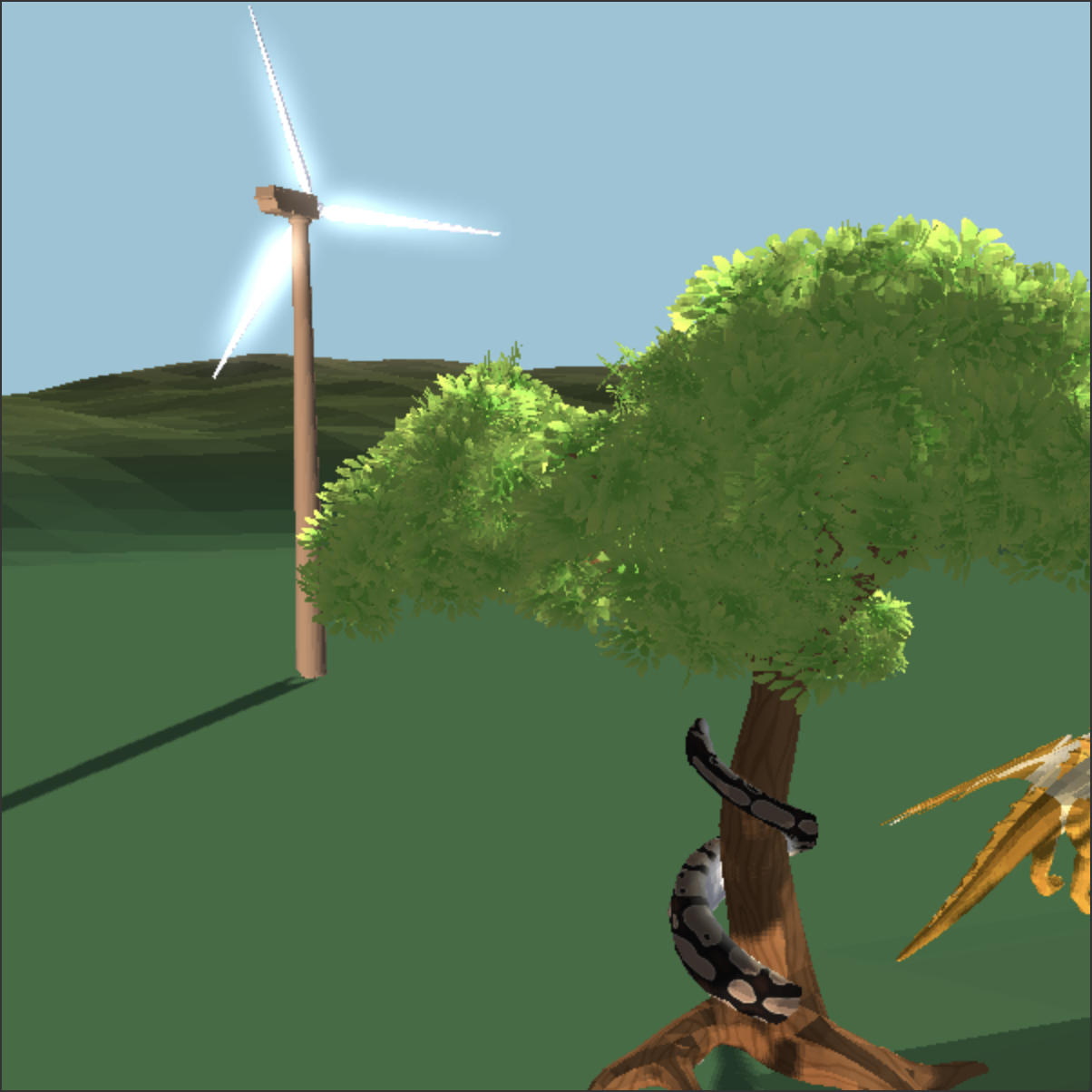
The course provided two python models: one straight and laid flat, and one coiled. I couldn’t quite get rid of a dissolve when morphing between the two models, so I computed the target coiled pose: a helical wrap of the straight model.
The python’s skeleton center is a simple unit circle in x and z climbing straight up along y:
// t = distance along python: t = 0 (tail) to t = 1 (head)
const theta = t * WRAP_TURNS * 2 * Math.PI;
const center = [
    WRAP_RADIUS * cos(theta),
    t * WRAP_HEIGHT,
    WRAP_RADIUS * sin(theta),
];
But a snake is also volume, and volume is preserved with the tangent-normal-binormal trick. Three local directions are computed on each point on the helical centerline:
// radially outward from the tree
const radial = [cos(theta), 0, sin(theta)];
// derivative of the helical centerline, the angle in which the snake is
// "traveling"
const tangent = norm3([
    -sin(theta) * WRAP_TURNS * 2 * Math.PI * WRAP_RADIUS,
    WRAP_HEIGHT,
    cos(theta) * WRAP_TURNS * 2 * Math.PI * WRAP_RADIUS,
]);
// cross => perpendicular to both the tangent and radial directions
const binormal = norm3(cross(tangent, radial));
The original snake coordinates have these roles:
vz              // position along the snake
vx              // one cross-section axis
vy - ymid       // other cross-section axis
And the target position is:
out.push(
    center[0] + vx * binormal[0] + (vy - ymid) * radial[0],
    center[1] + vx * binormal[1] + (vy - ymid) * radial[1],
    center[2] + vx * binormal[2] + (vy - ymid) * radial[2]
);
In vector notation:
target =
    center(t)
    + vx * binormal(t)
    + (vy - ymid) * radial(t)
Conceptually, the snake’s left-to-right “fatness” is along the binormal, and its bottom-to-top “height” is along the radial.
We exponentially ease (instead of instantly snap) the snake into this target position.
The day/night cycle
We measure how high the sun is with const hi = clamp01(g_sunDir[1] / SUN_PEAK); then construct its color:
g_sunColor = [
    1.00 * sunStr,
    lerp(0.42, 0.96, hi) * sunStr,
    lerp(0.16, 0.88, hi) * sunStr,
];
Near the horizon, hi is near zero and sun color is approximately (1.00, 0.42, 0.16) (strongly orange). When the sun is high, sun color is approximately (1.00, 0.96, 0.88) (a warm white).
The moon’s light is cool and blue:
const moonStr = 0.52 * moonUp;
g_moonColor = [
    0.55 * moonStr,
    0.62 * moonStr,
    0.90 * moonStr,
];
We similarly interpolate ambient light and the sky color between night and day.
Whichever of the sun or the moon is higher becomes the key light for casting shadows. The stars are faded in as g_nightness = 1.0 - dayness;.
Perlin terrain
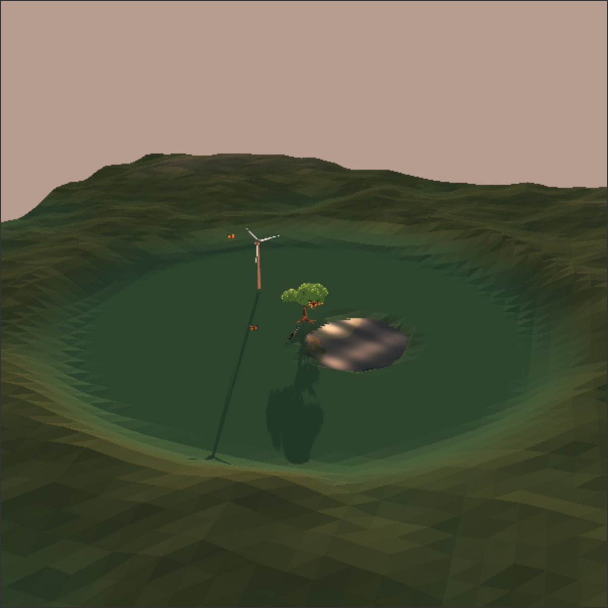
Calling the Perlin sampler four times at increasing frequencies lets us use noise across different “regimes”:
for (let o = 0; o < 4; o++) {
    sum += amp * g_noise.perlin2(
        x * freq + 100.0,
        z * freq + 100.0
    );
    norm += amp;
    amp *= 0.5;
    freq *= 2.0;
}
This is the fractal Brownian motion trick. The highest-amplitude, lowest-frequency octaves produce tall, broad hills; the lowest-amplitude, highest-frequency octaves produce low, small bumps.
A land point’s altitude lets us infer its color:
const valley = [0.26, 0.47, 0.28];  // grassy, green
const slope  = [0.34, 0.40, 0.20];  // olive
const peak   = [0.56, 0.50, 0.38];  // tan, rocky
// color is interpolated as t in the two intervals valley->slope and slope->peak
const t = clamp(y / HILL_HEIGHT);
Billboarding
We rotate the butterflies, and the sun and the moon so that they always face the camera. This cheaply makes them look 3D. Specifically, for the butterfly, we have a faceCameraMatrix() that computes the direction from the butterfly to the camera:
const ny = norm3([
    cam[0] - p[0],
    cam[1] - p[1],
    cam[2] - p[2],
]);
The butterfly’s local +Y axis is normal to its wings, so ny always faces the camera. We compute the +Z direction from body towards the head:
let up = [0, 1, 0];     // up-world direction
const d = dot(up, ny);  // projection onto the camera-facing direction
const nz = normalize(   // butterfly-local "up"
    up - d * ny
);
This gives us the final perpendicular axis for free:
const nx = cross(ny, nz);
Billboarding is especially important for the sun and the moon; without it, they’d look like ellipses when viewed from an angle instead of flat discs.
Nailing stars to the wall
Stars are randomly generated gl.POINTS whose node is translated to the camera position as
n.localMatrix = new Matrix4().setTranslate(
    g_cameraEye[0],
    g_cameraEye[1],
    g_cameraEye[2]
);
so that moving the camera doesn’t make the viewer approach the stars while still changing screen position when the camera rotates. The sun and the moon also use a similar camera translation trick. This is the cheap approximation of what a principled skybox would give you.
-
Fascinatingly, the folk explanation that this is due to evolution catching retinas up to the fact that green plants are food is probably wrong — vertebrates had long-wave opsins long before terrestrial plants were anybody’s food, and amino-acid biochemistry simply happens to put the M and L absorption peaks around 550-560 nm. Yellow-green senstivity is, incidentally, why simple saturation/value (e.g., a pure red
(255, 0, 0)) doesn’t produce “neon”: 550-560 nm is the most neon band of RGB partly because of the human eye’s heightened sensitivity to it, and it’s why some modern fire trucks are lime-green. Color spaces that are aware of this and other quirks of the human visual system (CIELAB and its increasingly sophisticated descendants) are frequently used in UI design. ↩