The Illustrated Hyena

Attention is great for language modeling, but has a steep computational cost: as the sequence length $\mathrm{L}$ grows, the cost grows quadratically (attention is $\mathcal{O}(\mathrm{L^2})$). This can make powerful applications impractical: using entire textbooks or reams of technical documentation as context, generating long-form music and video, or processing gigapixel-scale images. Hyena is a subquadratic attention alternative potentially unlocking those applications: it’s $\mathcal{O}(\mathrm{L \log L})$. Recently, it was used in Arc Institute’s genomic language model Evo (which made the Science cover) to help model inter-gene relationships over long distances. Evo is trained on a context length of ~130,000 tokens, and can generate sequences with plausible high-level architecture more than 1 million tokens in length.

This post is a breakdown of the Hyena operator’s architecture. It’s based primarily on the 2023 paper introducing Hyena. Like Illustrated Transformer and Illustrated AlphaFold, I aim to use lots of visualizations.

Here’s an outline:

• A walkthrough of the matrix math to show how the computational cost of attention grows quadratically ($\mathcal{O}(\mathrm{L^2})$) with the sequence length.
• A few subquadratic attention alternatives ML researchers have developed over the years and where they fall short.
• The $\mathcal{O}(\mathrm{L \log L})$ Hyena algorithm proper.
• Four of Hyena’s key properties:
  • It’s a data-dependent operator, meaning that the input sequence undergoes a transformation that depends on the input itself. Hyena shares this feature with attention, where the projection V of the input is transformed using an attention pattern that is in turn derived from projections of the input.
  • Hyena’s parameter count is independent of the sequence length.
  • There’s no architecture-imposed upper limit on its context window.
  • Hyena has an inductive bias that weights local context more highly.
• Hyena’s empirical results on language (and vision) modeling.

Here’s a TL;DR of the Hyena algorithm:

Successively apply fast Fourier transform-based long convolutions and elementwise multiplications with projections of the input sequence. To avoid storing long filters in memory, implicitly parametrize them with feedforward networks.

We will unpack what all that means.

Here’s the background I assume:

• Basic linear algebra (like knowing how matrix multiplication works)
• A high-level understanding of what feedforward networks/MLPs and CNNs do
• The first two sections require understanding how the attention mechanism works. But
  • the first section has plenty of refreshers, as well as links to more in-depth resources, and
  • you can skip the first two sections if you’re prepared to accept their top-level claims: Attention is $\mathcal{O}(\mathrm{L^2})$. Folks have been trying workarounds.

Here’s a table of contents:

• The problem with attention
  • Projecting into Q, K and V
  • Computing the attention matrix
  • Computing the attention pattern
  • Multiplying the attention pattern and V
  • Concatenation, projection and addition to the residual stream
  • Recap
• The search for subquadratic attention alternatives
• The Hyena algorithm
• Hyena is a data-controlled operator
• Hyena has sublinear parameter scaling and unrestricted context
• Hyena filters have an inductive bias of locality
• Empirical results
• Conclusion

The problem with attention

This section has some refreshers but mostly assumes familiarity with how attention works. If you want an introduction to attention, check out one of these resources, ordered by time commitment:

• 3Blue1Brown’s ~30-minute video and his ~1-hour lecture,
• Jay Alammar’s Illustrated Transformer,
• Brendan Bycroft’s visualization,
• Harvard NLP’s Annotated Transformer, and
• ARENA’s code-your-own-transformer-from-scratch guide.

Attention’s quadratic asymptotic complexity comes from exactly three steps: computing the attention matrix QK^T, softmaxing the attention matrix’s rows to get the attention pattern, and multiplying the attention pattern with V. We’ll walk through each step of the attention mechanism to show this. If you’re happy with this top-level summary, though, feel free to move on to the next section.

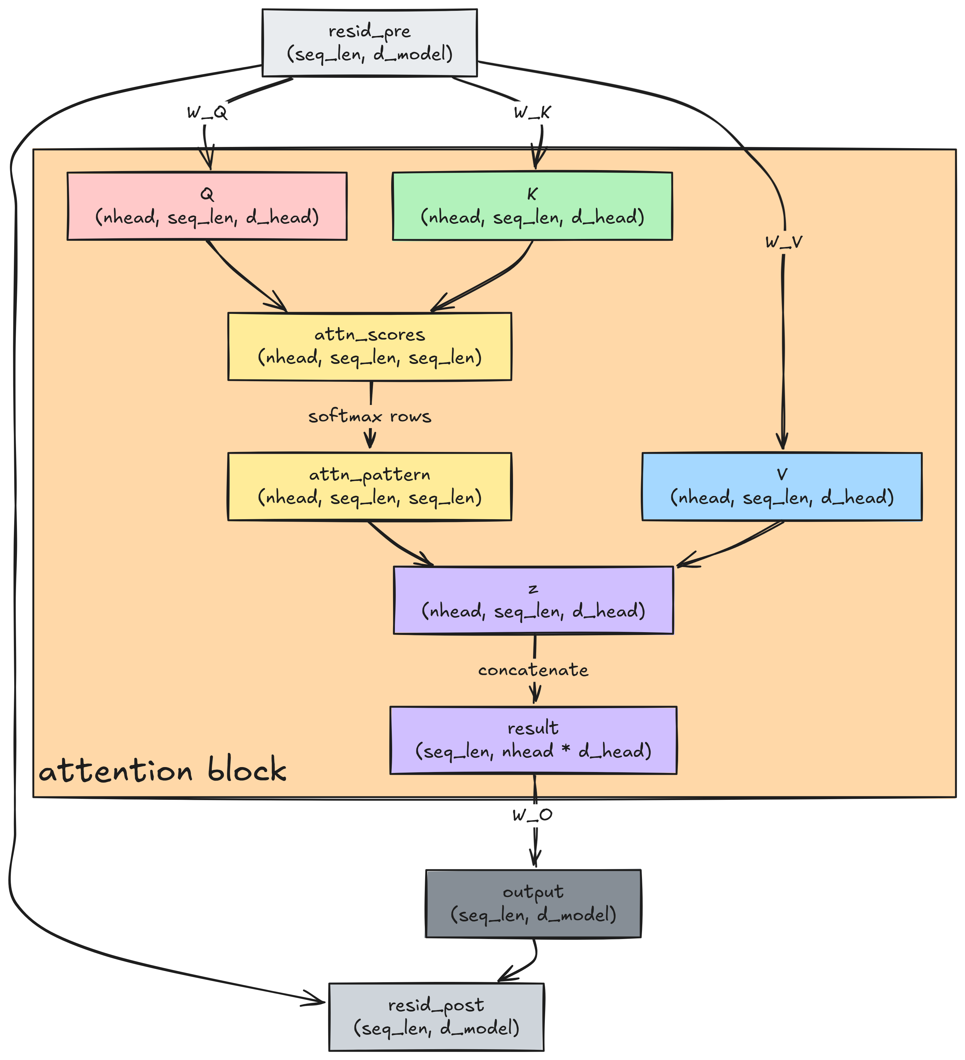Adapted from ARENA

Projecting into Q, K and V

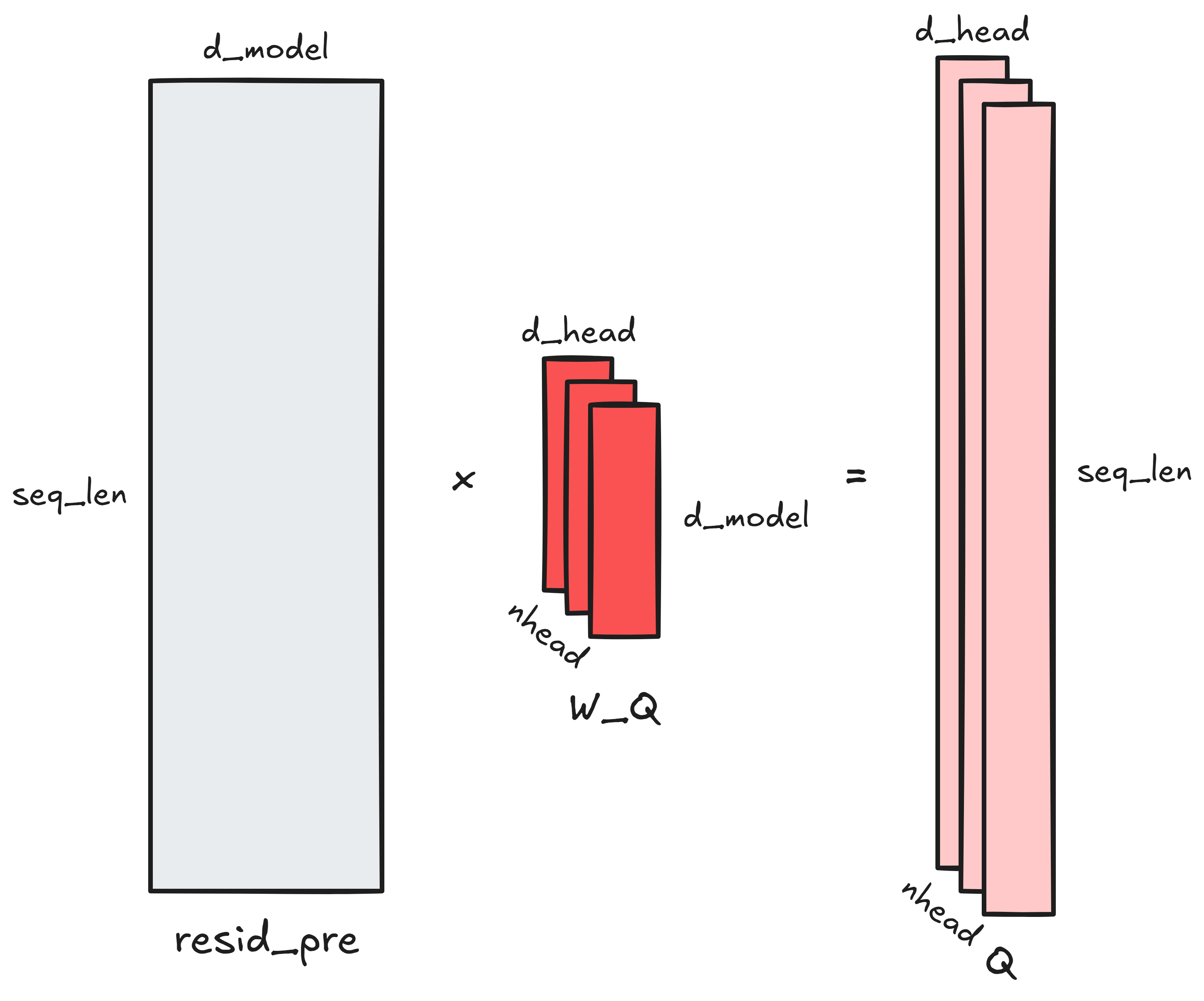
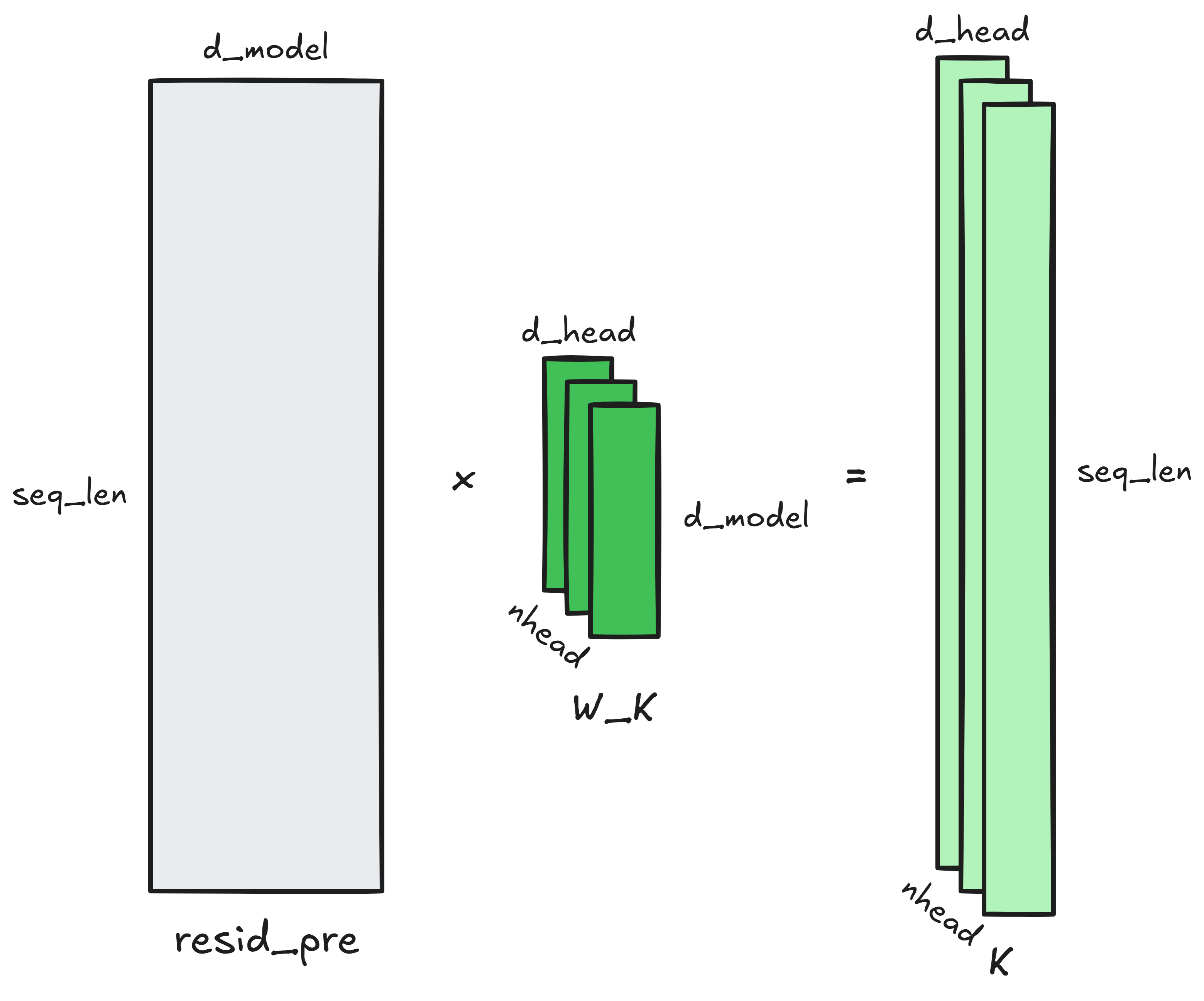
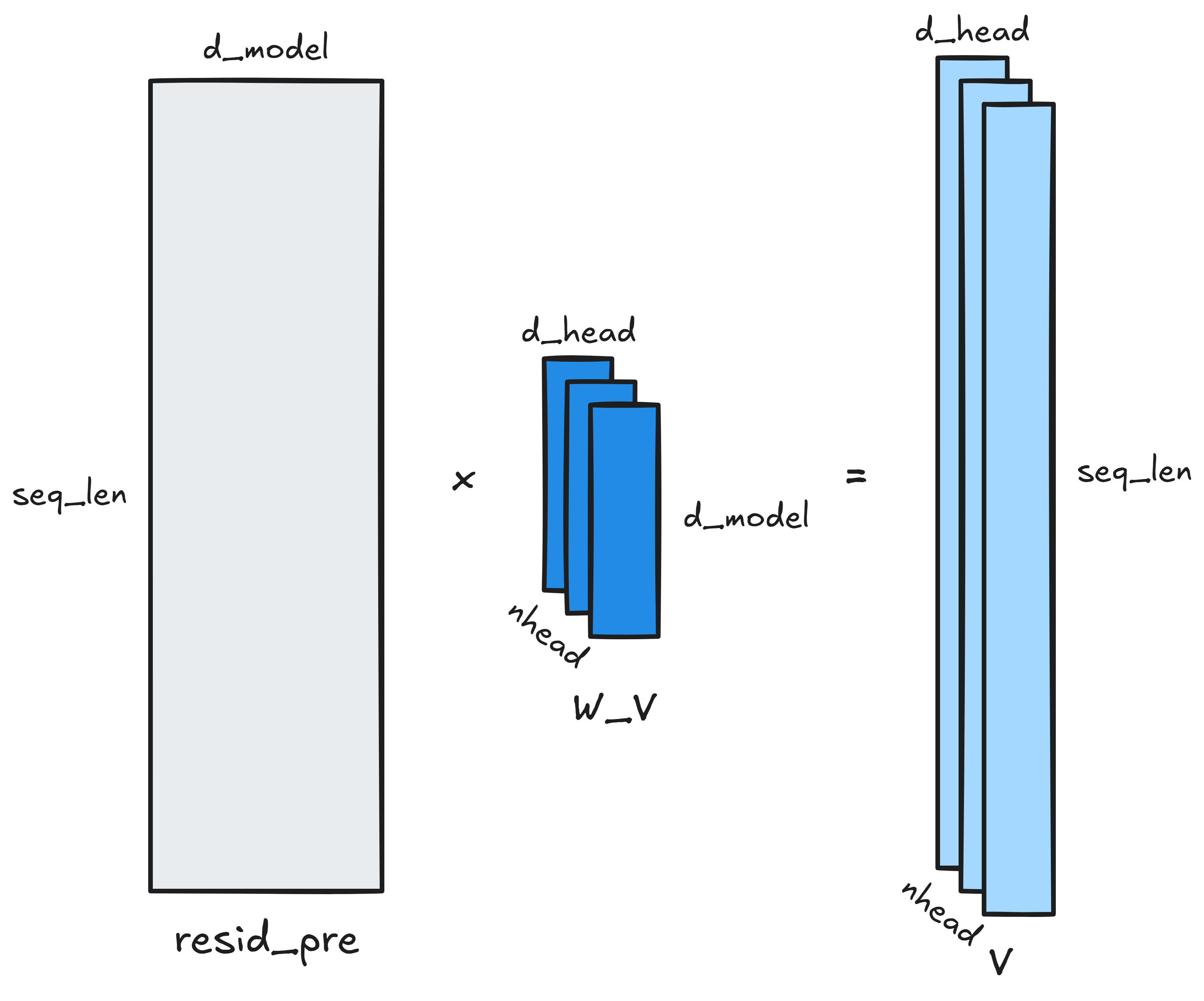
The input to an attention block is the (seq_len, d_model) residual stream. The first step is projecting it (almost always) down to nhead triplets of Q, K and V matrices. Each of these matrices is of dimensions (seq_len, d_head): the seq_len vectors go from dimension d_model to dimension d_head. (Usually, the nhead Q matrices are written together as a single (nhead, seq_len, d_head) matrix. Ditto for the K and V matrices: they’re written as big (nhead, seq_len, d_head) matrices. This allows vectorized operations. But as the excellent Mathematical Framework for Transformer Circuits notes, the matrix representation most amenable to blazing fast matmuls is not necessarily the easiest to understand. I find it helpful to think of the Q, K and V projections not as three monolithic (nhead, seq_len, d_head) matrices, but as nhead triplets of (seq_len, d_head) matrices: one triplet of projected-down representations of the residual stream for each head.)

nhead triplets of learned matrices are responsible for these projections: call them W_Q, W_K and W_V for the Q, K and V projections respectively. Each transforms the (seq_len, d_model) residual stream to a (seq_len, d_head) representation. So, W_Q, W_K, and W_V are each of dimensions (d_model, d_head).

Each projection from d_model to d_head is of complexity

where $L$ is seq_len.

Why? Think of it this way: each entry in the (seq_len, d_head) output matrix is a dot product between d_model-dimensional vectors (in more literal terms: an elementwise multiplication of a row of the (seq_len, d_model) residual stream with a column of the (d_model, d_head) W_Q, W_K or W_V). This involves multiplying d_model pairs of scalars, then summing the d_model pairwise products. That’s an $\mathcal{O}(\mathrm{d\_model})$ operation repeated for each of the $\mathrm{L \cdot d\_head}$ entries of the (seq_len, d_head) output: $\mathcal{O}(\mathrm{L \cdot d\_head \cdot d\_model})$, all told.

In general, if you’re multiplying an $m \times n$ matrix by an $n \times p$ matrix, it’s an $\mathcal{O}(m \cdot n \cdot p)$ operation. Notice how each of the $mp$ cells in the output is a sum of $n$ pairwise products:

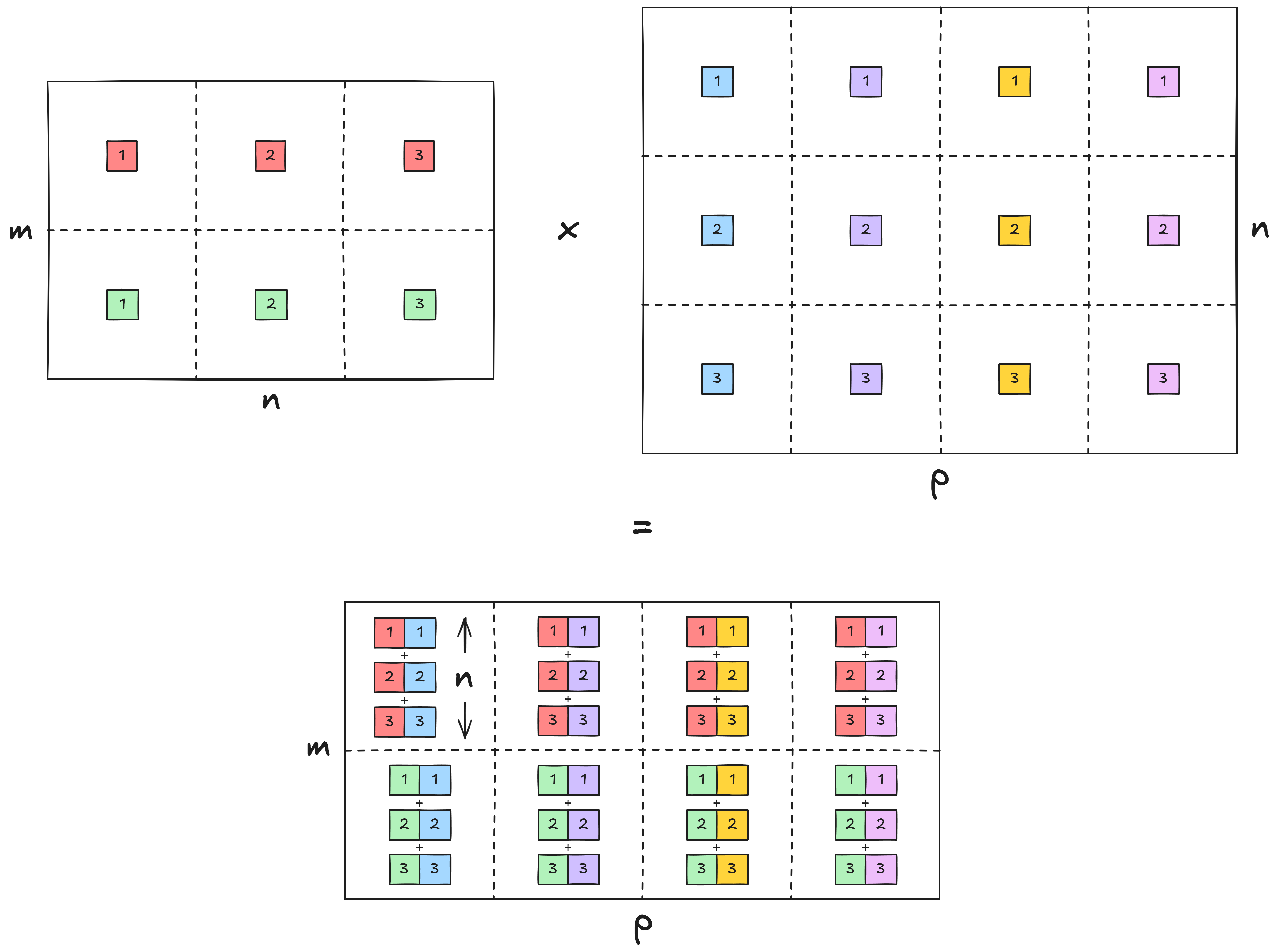
In code, if you’re multiplying (m, n) A and (n, p) B:

for row in range(m):
    for col in range(p):
        output[row][col] = 0
        for i in range(n):
            output[row][col] += A[row][i] * B[i][col]

That’s one addition for each of the n iterations of the innermost loop. In the loop just around the innermost loop, you perform on the order of n operations per iteration for p iterations. Finally, in the outermost loop, which goes on for m iterations, you perform n * p operations per iteration. That’s a total of m * n * p operations.

There are $3 \cdot \mathrm{nhead}$ projections of the residual stream in a single multi-headed attention block (3 per head, and nhead heads). So, the overall computational complexity is

But notice that $3$, $\mathrm{nhead}$, $\mathrm{d\_head}$ and $\mathrm{d\_model}$ are fixed hyperparameters. Constants are dropped from complexity analysis. The complexity of this step is simply

The initial projections are of linear complexity.

Computing the attention matrix

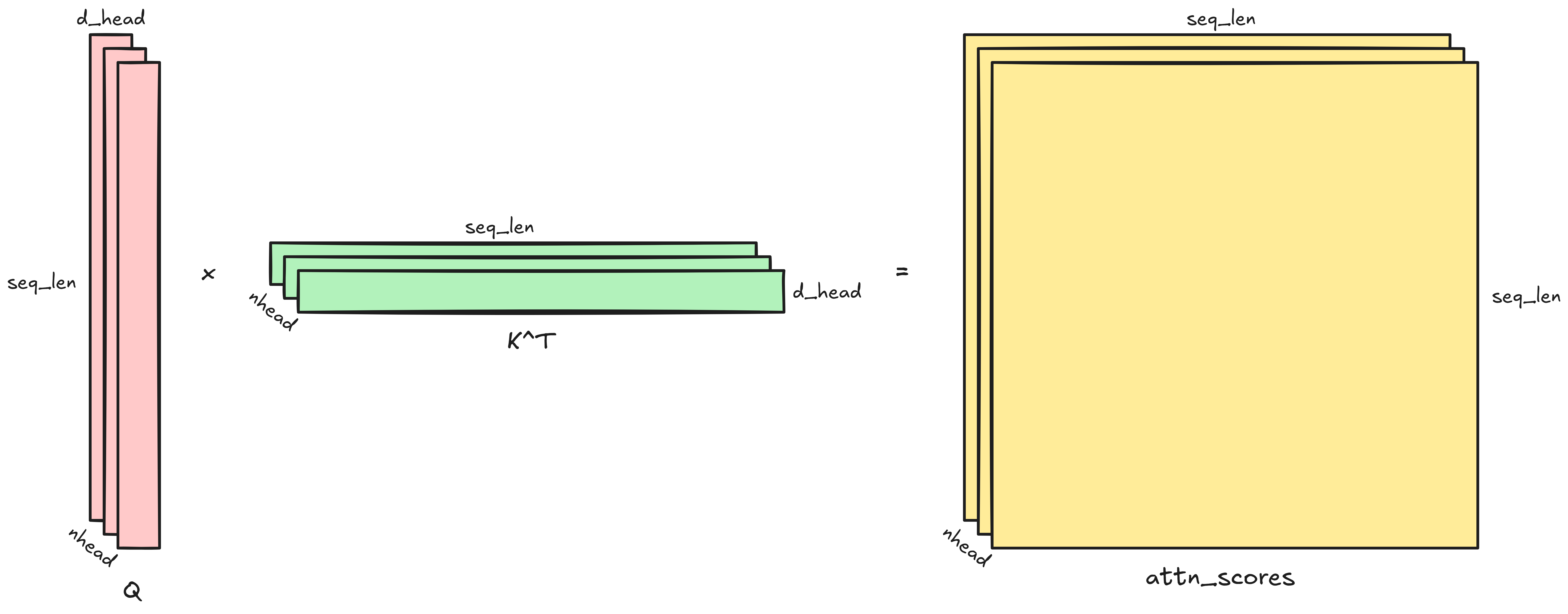
Once we have Q and K, we need to compute QK^T. In other words, we need to multiply a (seq_len, d_head) matrix with a (d_head, seq_len) matrix. The output will be the (seq_len, seq_len) attention matrix. Each entry of the attention matrix is a dot product between d_head-dimensional vectors. The computational complexity is

per head (each entry of the (seq_len, seq_len) output is the dot product of d_head-dimensional vectors).

With nhead heads per attention block, the complexity of multi-headed attention is

Dropping constants as before, the complexity of generating the attention matrices across the attention block is

Computing the attention matrix is of quadratic complexity.

Already, we can see that attention has become quadratic with the sequence length. We can stop here, since we’ve found that the complexity of attention is at least quadratic: a program is bottlenecked by its slowest subroutine. But for the sake of completeness, and for locating other, less well-known sources of quadratic complexity, let’s continue.

Computing the attention pattern

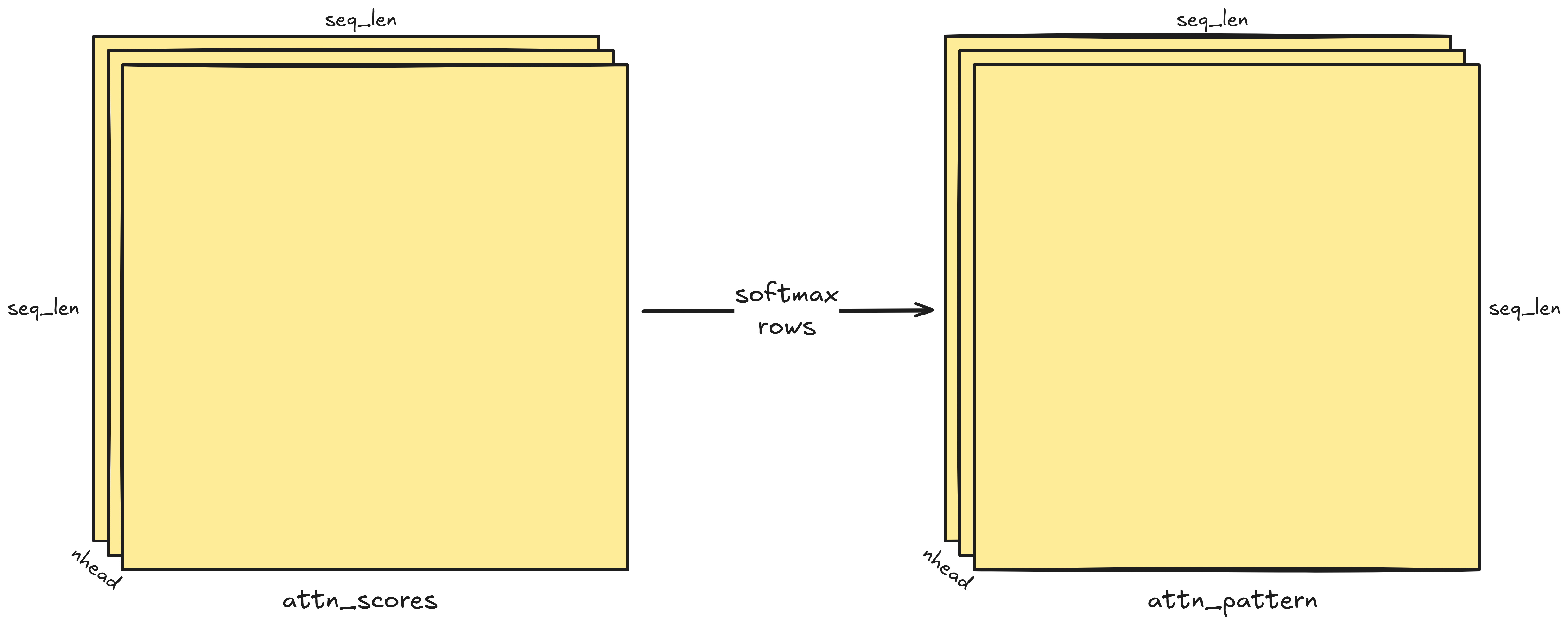
We softmax the rows of the attention matrix to get the attention pattern. Recall the softmax function:

For every row, we need to:

• find its maximum entry and subtract it from each entry in the row for numerical stability (incurring a computational cost linear with the row length),
• exponentiate each entry in the row (linear),
• sum the exponents to calculate the denominator (linear), and finally
• divide each exponentiated entry by the sum of the exponents (linear).

That’s $\mathcal{O}(\mathrm{L})$ operations for each of the $\mathrm{L}$ rows, or

for the entire attention matrix.

For nhead heads:

Dropping constants and keeping just the dominant term:

Computing the attention pattern is of quadratic complexity.

Multiplying the attention pattern and V

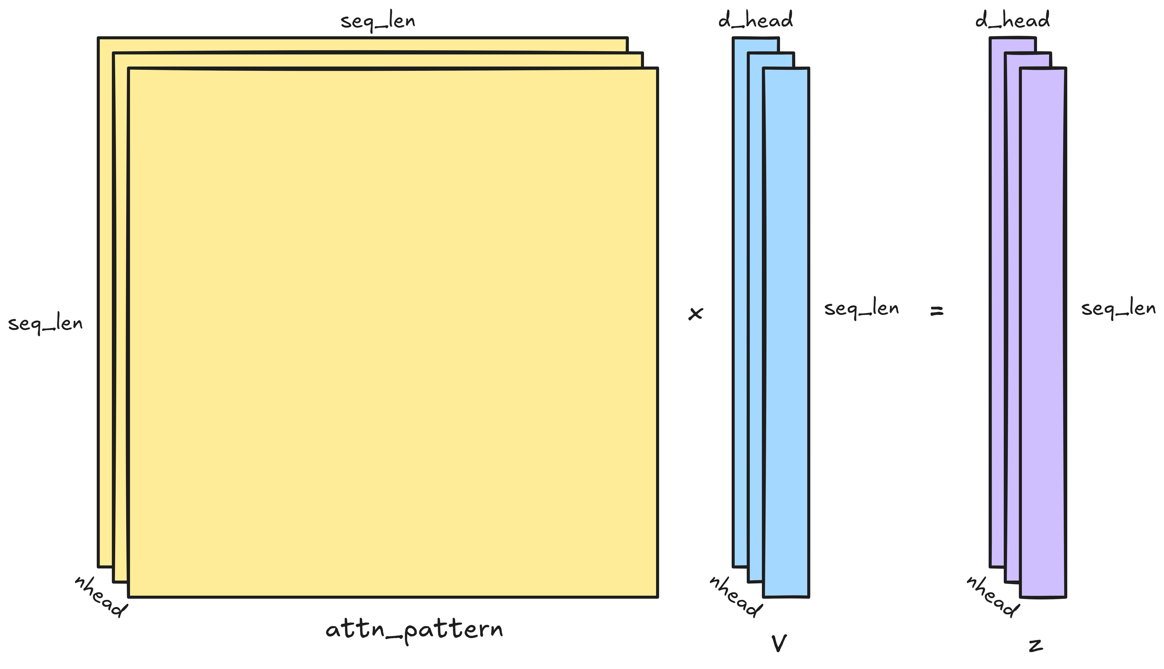
We now have a (seq_len, seq_len) attention pattern and a (seq_len, d_head) V for every head. Multiplying them is of complexity

since each entry of the (seq_len, d_head) output matrix is a dot product of seq_len-dimensional vectors. There are nhead of these matrix multiplications in an attention block:

But after dropping the constants $\mathrm{nhead}$ and $\mathrm{d\_head}$:

Multiplying the attention pattern and V is of quadratic complexity.

Concatenation, projection and addition to the residual stream

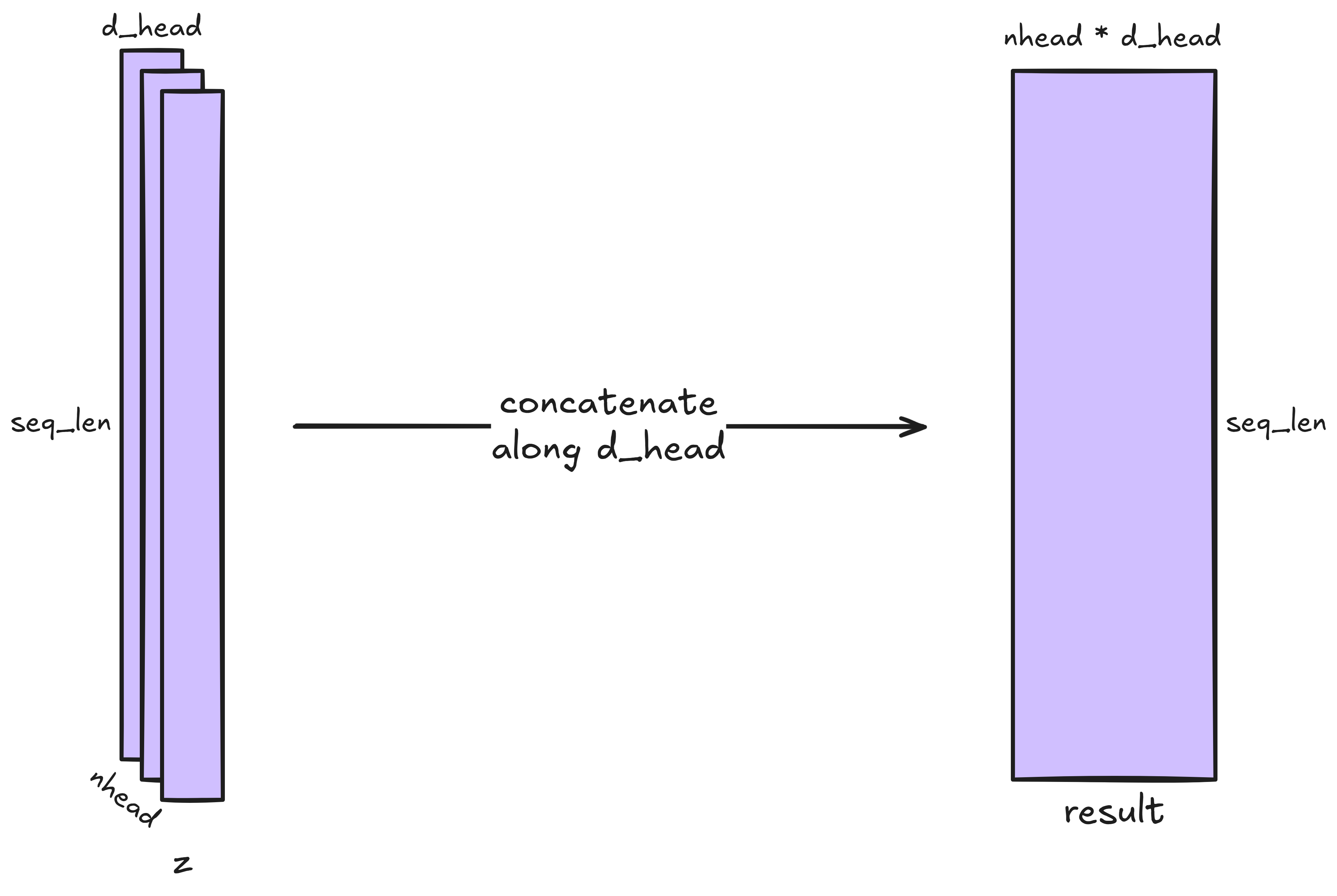
The nhead (seq_len, d_head) matrices are first concatenated into a single (seq_len, nhead * d_head) matrix. This requires moving every entry of nhead (seq_len, d_head) matrices into a new, larger matrix. Since we must touch every entry exactly once, the computational complexity is

or simply

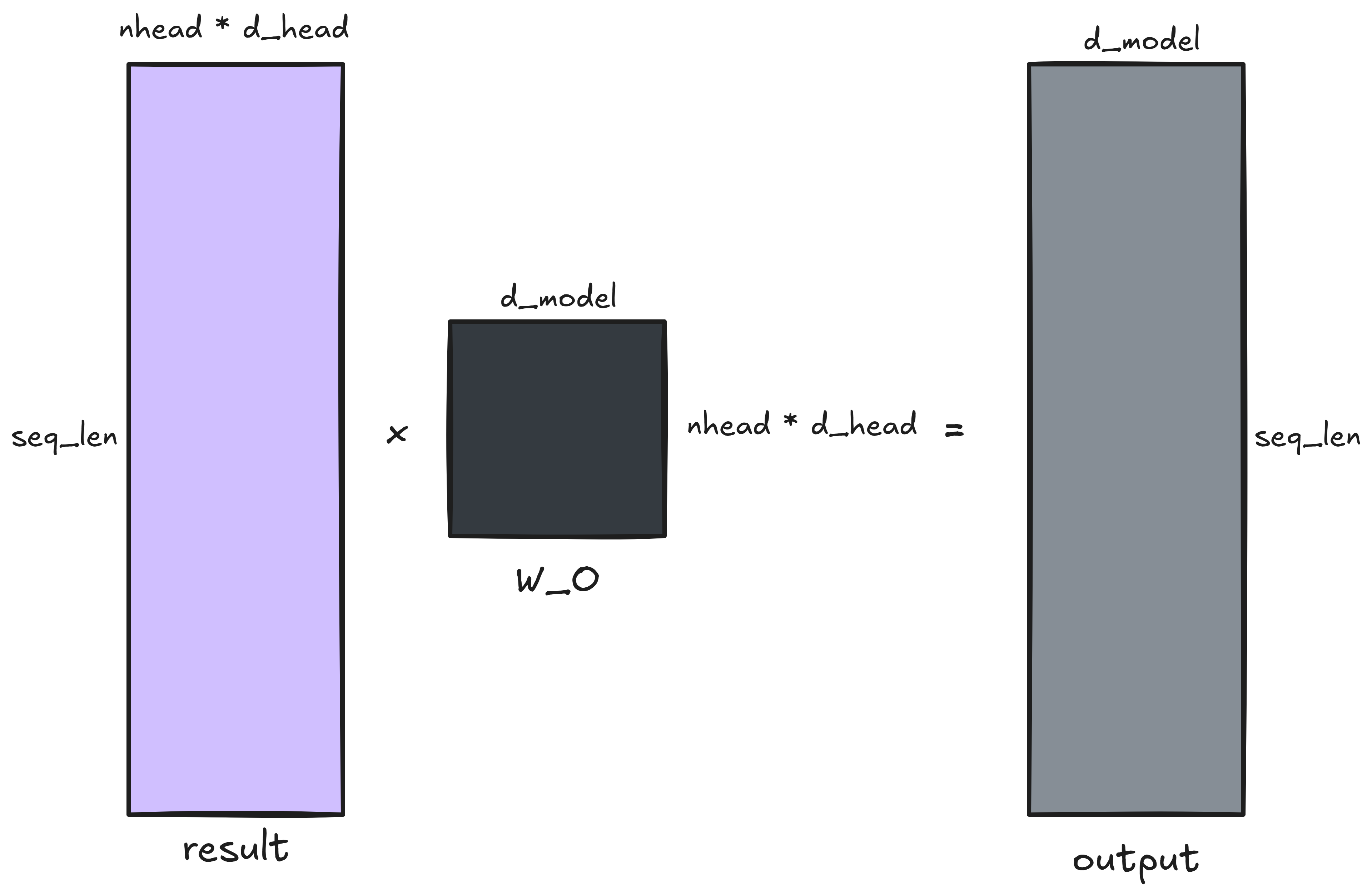
This (seq_len, nhead * d_head) concatenated matrix is projected to a (seq_len, d_model) matrix. Each entry of the output (seq_len, d_model) matrix is a dot product of nhead * d_head-dimensional vectors, so this step is of complexity

or simply

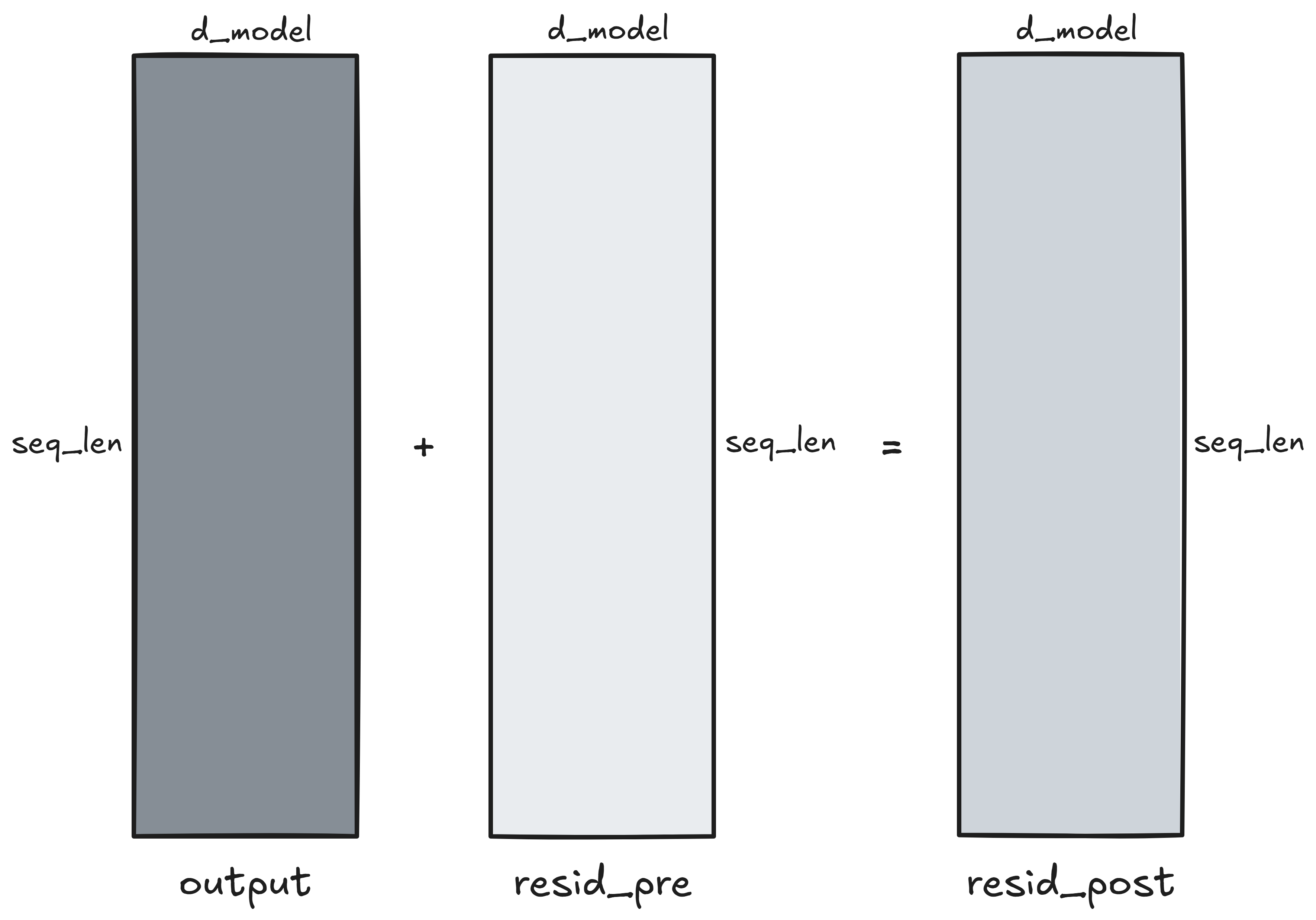
This matrix is finally added to the residual stream. Each entry of the output (seq_len, d_model) matrix is a sum of 2 entries. The complexity is

or simply

Concatenating, projecting and adding the output to the residual stream is of linear complexity.

Recap

These steps are of quadratic complexity:

• Computing QK^T, the attention matrix.
• Softmaxing the rows of the attention matrix to get the attention pattern.
• Multiplying the attention pattern and V.

These steps are of linear complexity:

• Initial projections of the input sequence into Q, K and V.
• Concatenating, projecting and adding the output to the residual stream.

The search for subquadratic attention alternatives

The quadratic complexity of attention is bad news. As the Hyena paper puts it, and as I noted in the introduction, the cost could prohibit using “entire textbooks as context, generating long-form music or processing gigapixel scale images”.

Yet, natural language processing doesn’t have to be quadratic. A whimsical argument: take humans. We don’t make comprehensive pairwise word comparisons while writing text. Instead, we build up an internal knowledge state, RNN-like. We are an existence proof of subquadratic, generally intelligent language processing.

If we can build a subquadratic attention alternative, we’d also like it to be drop-in: i.e., allowing us to swap out the attention mechanism for our new operator with minimal changes to the rest of the transformer architecture. This would let us carry over many of the algorithmic/hardware advancements we’ve already made, and make it easier to engineer the operator into models.

The subquadratic attention alternative literature is huge and documented well in this survey. And yet, as the survey notes, none of the alternatives have replaced vanilla attention as the de facto standard. Each drop-in replacement seems to be deficient in its own way.

Take Linformer. This approach theoretically achieves $\mathcal{O}(\mathrm{L})$ complexity by projecting the (seq_len, d_head) K and V matrices down to (k, d_head) matrices. Here, k is a fixed hyperparameter (as you’d expect, bigger k generally means better performance). We multiply (seq_len, d_head) Q and (d_head, k) K^T to get the attention matrix. So, the attention matrix is of dimensions (seq_len, k).

Each entry of the (seq_len, k) attention matrix is a dot product of d_head-dimensional vectors. So, the complexity is

or simply

Linear, not quadratic! The problem? Linformer and its other linear-complexity cousins seem to perform worse at downstream tasks, or take much more compute, than even a very simple efficient sparse architecture. Plus, they can be a pain to do causal masking on.

Some other attention alternatives aim to sparsify the attention matrix. That is, they aim to get away with computing just a few key pairwise weights in the attention matrix instead of every weight.

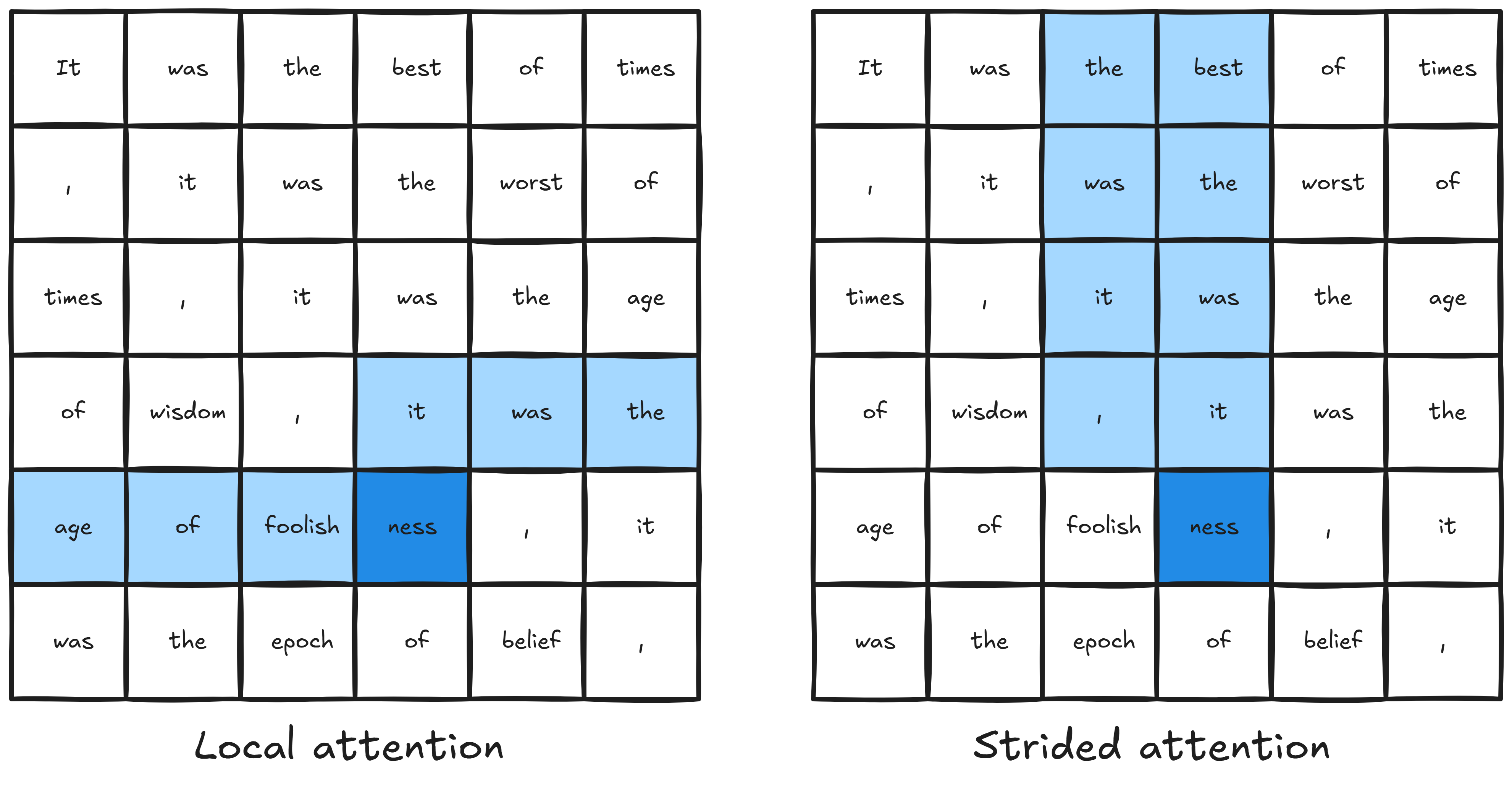
OpenAI’s Sparse Transformer, which arguably kicked off the efficient transformer research direction, takes this approach. It achieves a theoretical computational complexity of $\mathcal{O}(\mathrm{L \sqrt{L}})$.

To see how it works, imagine the input sequence being divided into $\sqrt{\mathrm{L}}$ blocks, each with $\sqrt{\mathrm{L}}$ tokens. Half the attention heads attend to a block of just the previous $\sqrt{\mathrm{L}}$ tokens — call these the “local” heads. The other half attend to a fixed number of tokens from each of the $\sqrt{\mathrm{L}}$ blocks (you can think of these tokens as “summarizing” their blocks’ contents) — call these the “strided” heads.

In the local heads, each row attends to $\sqrt{\mathrm{L}}$ tokens and there are $\mathrm{L}$ rows, so the computational complexity is $\mathcal{O}(\mathrm{L} \sqrt{\mathrm{L}})$. In the strided heads, each row attends to $c$ tokens each from $\sqrt{\mathrm{L}}$ blocks, or $c \sqrt{\mathrm{L}}$ tokens in all. There are $\mathrm{L}$ rows. So, the computational complexity is again $\mathcal{O}(\mathrm{L} \sqrt{\mathrm{L}})$ (dropping the constant $c$, which is often small compared to the sequence length).

The overall complexity of sparse attention is $\mathcal{O}(\mathrm{L \sqrt L})$.

Sparse attention has seen some use. Most famously, the only architectural difference between GPT-3 and GPT-2 was that the former used “alternating dense and locally banded sparse attention patterns in the layers of the transformer”. However, on its own, the sparse transformer seems to perform notably worse than the vanilla transformer.

It is in this research tradition of attempting to outrun attention that Hyena is placed. However, it is different from many of its predecessors in that it doesn’t try to approximate the attention matrix at all.

The Hyena algorithm

In this section, we go over the $\mathcal{O}(\mathrm{L \log L})$ algorithm for Hyena, which is a drop-in attention alternative.

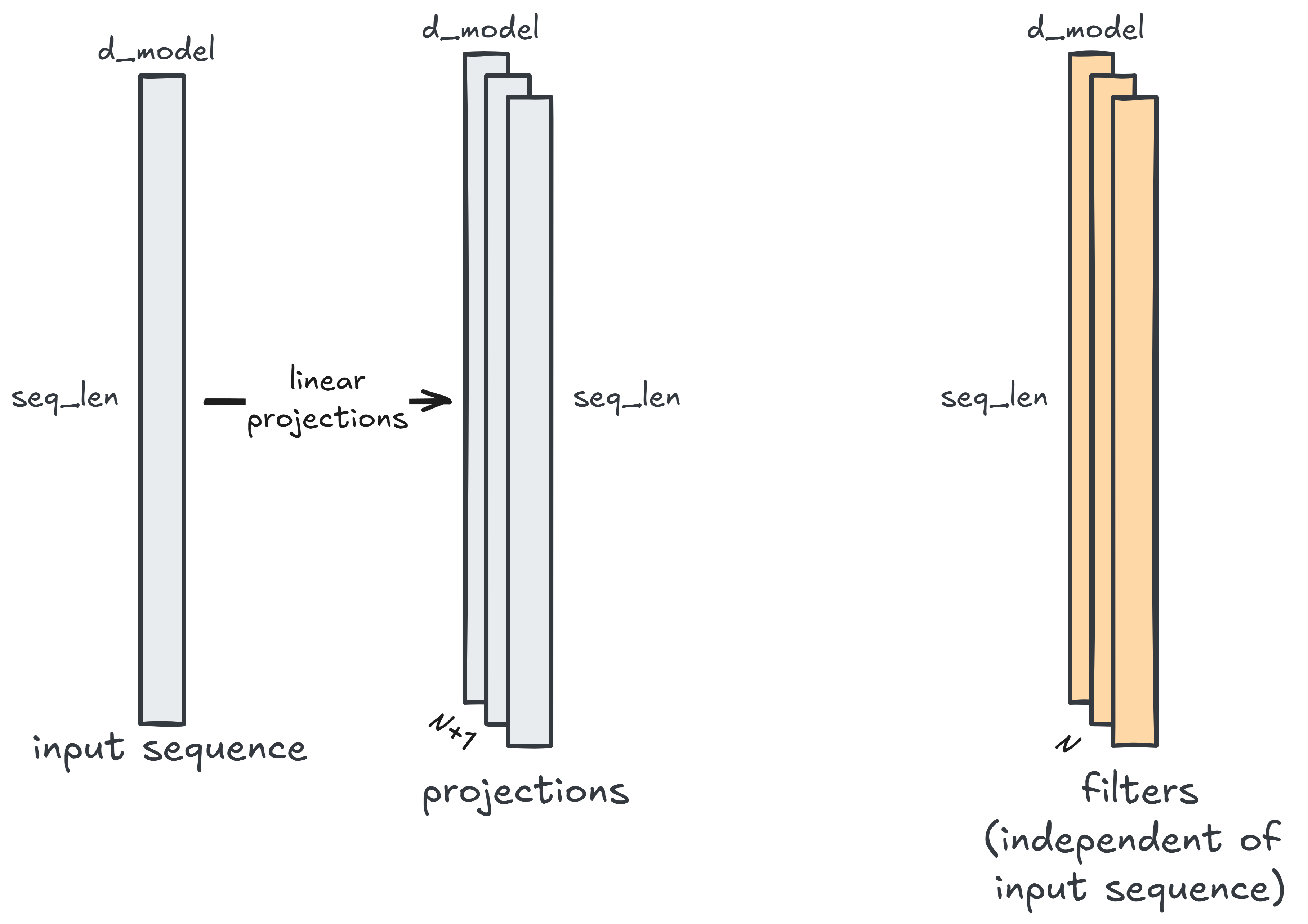
First, we transform the (seq_len, d_model) input sequence into $N+1$ (seq_len, d_model) linear projections (to emphasize: same sequence length, same embedding dimension). (Why we’re singling out the $+1$th projection will become clear in a bit. For now, just note there are $N+1$ linear projections.) This is similar to the first step in the attention mechanism: linear projection of the input sequence into Q, K and V matrices that are each as long as the input sequence. Two key differences: First, Q, K and V typically have d_head-dimensional vectors where d_head is essentially always smaller than d_model. Not so in Hyena: each of the $N+1$ projections has the same embedding dimension d_head as the input sequence. Second, $N+1$ need not be three (unlike attention’s Q, K and V).

Next, Hyena generates $N$ convolutional filters that are each as long as the input sequence. Notice the significant departure from convolutional filters you may be familiar with. In CNNs, filters are small compared to the image:

In MNIST, for example, you typically do 3 x 3 or 5 x 5 filters versus 28 x 28 MNIST images. This is by design: CNNs exploit an inductive bias of localizable features like edges and color splotches. Similarly, 1D convolutional filters in certain sequence prediction models (like time-series) exploit an inductive bias of localizable patterns (like swings, crashes, and bull runs). 1D convolutional models used for text processing too turn out to develop “comparative kernels” including "as ... as" and "of more than" patterns, “spokesman kernels” which detect "a <company> spokesman", kernels detecting occupations like "chief economist john" and "exchange chairman john", and more kernels detecting short phrasal patterns.

You can think of these smaller filters as doing short convolutions, as opposed to Hyena’s long convolutions. The convolution algorithm making use of these filters is the same we know and love: slide the filter over the input, elementwise multiply overlapping values, sum the elementwise products to obtain a single value of the output. It’s just the length of the filter that’s unusual. Here’s a visualization of a long convolution (yellow for the filter, blue for the sequence):

To recap: we now have $N+1$ projections of the input and $N$ long filters.

Of the $N+1$ projections, pick one and call it v. We convolve v with one of the filters we just generated, then elementwise multiply it with another one of the $N+1$ projections. Repeat $N$ times. (This explains why we had $N+1$ projections: $N$ projections are used for the multiplicative updates while the $+1$th projection is the initial value v.)

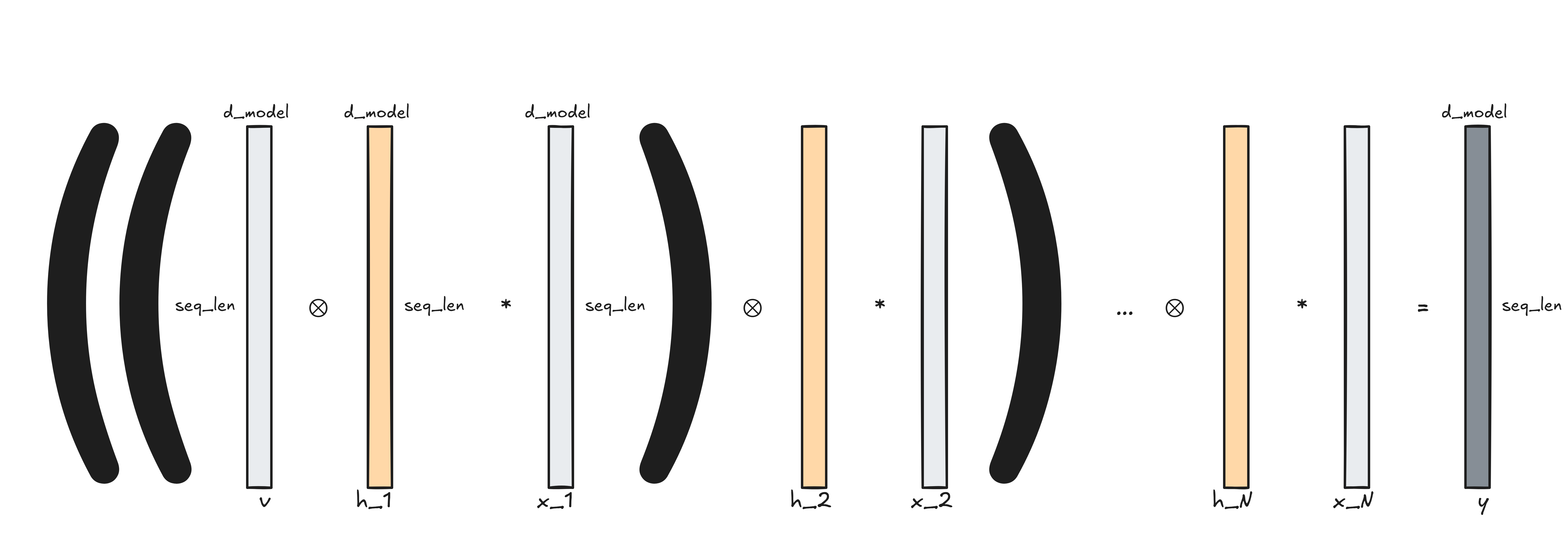
Let’s call the $N+1$ projections v and x_1, x_2, …, x_N, and the filters h_1, h_2, …, h_N. We’ll represent elementwise multiplication using the * operator (borrowing from numpy and PyTorch). Then, here’s what the pseudocode looks like:

z = v
for i in range(N):
  z = x_i * convolve(h_i, z)
return z

z can be rewritten as

z = (((((v ⊗ h_1) * x_1) ⊗ h_2) * x_2) ... ⊗ h_N) * x_N

(The circled asterisk ⊗ is convolution and the asterisk * is elementwise multiplication.)

Here’s a visualization of what’s going on:

Now that we have a broad outline of the algorithm down — convolve and elementwise multiply with a projection of the input, repeat $N$ times — we can move on to analysis of its computational complexity:

• Let’s look inside the loop. Naively, the computational complexity of the convolve() operation is $\mathcal{O}(\mathrm{L}^2)$. Why? Because each value of the $\mathrm{L}$-long output is the dot product of (on the order of) $\mathrm{L}$-long vectors. But if you use something called the Cooley–Tukey fast Fourier transform (FFT), you can bring this down to $\mathcal{O}(\mathrm{L \log_2 L})$! (Understanding why will require knowing Fourier theory first, the convolution theorem next, and then the FFT algorithm proper. I’m afraid that’s outside the scope of this post — but it’s fine to treat the FFT as a black box that makes convolutions faster.) Henceforth, we’ll assume a base of $2$ and just write $\log$.
• Next, we do an elementwise multiplication. That’s $\mathcal{O}(\mathrm{L})$ because you’re multiplying each of a sequence’s $\mathrm{L}$ entries with corresponding entries from another $\mathrm{L}$-long sequence.
• The news so far: we have an $\mathcal{O}(\mathrm{L \log L})$ convolution followed by an $\mathcal{O}(\mathrm{L})$ elementwise multiplication inside the for loop.
• The for loop goes on for $N$ iterations. So, we’ve got ourselves an $\mathcal{O}(N\mathrm{(L \log L + L)}) = \mathcal{O}(N\mathrm{(L \log L)})$ algorithm (we drop the $+ \mathrm{L}$ because $\mathrm{L \log L}$ dominates).

Note that there’s a bit of subtlety in the constants-included computational complexity. The loop must convolve across every one of the d_model embedding dimensions. This means that the complexity is actually $\mathcal{O}(ND\mathrm{(L \log L)})$. In practice, of course, $N$ and $D$ are fixed hyperparameters and the asymptotic complexity is simply $\mathcal{O}(\mathrm{L \log L})$ (better than vanilla attention’s $\mathcal{O}(\mathrm{L^2})$!). The constants are there just to make it a bit more precise what’s going on.

Though Hyena is theoretically faster than attention, in practice it runs faster than optimized attention only on sequences over 4096 tokens long. This is because Hyena’s GPU utilization is lower; but the authors “expect the gap between theoretical maximum speedup to shrink with improved implementations of FFTConv and specialized hardware”. FlashFFTConv is a step in that direction.

But does Hyena perform as well as attention? Before getting to the empirical results, let’s look at some neat theoretical features Hyena shares with attention.

Hyena is a data-controlled operator

Attention is special: it is a data-controlled linear operator.

First, let’s use a few examples to sketch out the general concept of a data-dependent transformation: imagine multiplying a matrix $A$ by

• a random matrix: that’s a data-independent transformation of $A$. The values of the random matrix don’t depend on the values of $A$.
• the identity matrix: that’s also a data-independent transformation. The values of an identity matrix stay the same regardless of what the values of $A$ are.
• the transpose of $A$, $A^T$: that’s taking $A$ through a data-dependent transformation. The transformation $A^T$’s values depend on the values of $A$ (since $A^T$ is just $A$ reflected across a ray along the diagonal).
• a matrix learned through gradient descent, but otherwise fixed during inference: data-independent transformation. What I’ve described is a feedforward network, of course. The network itself was learned from examples (hopefully!) from the same distribution as $A$. But after training, the recipe for transforming $A$ is fixed. If the learned matrix turns out to be $\begin{bmatrix} 5 & 7 \\ 3 & 9 \end{bmatrix}$, it’s $\begin{bmatrix} 5 & 7 \\ 3 & 9 \end{bmatrix}$ no matter what the entries of $A$ are.

Attention is a data-dependent operator: a projection of the input sequence, V, undergoes a transformation (multiplication with the attention pattern) that is different for every input sequence (since the attention pattern is itself generated from projections of the input sequence). This way, as the paper puts it, attention “[encodes] an entire family of linear functions in a single block”. 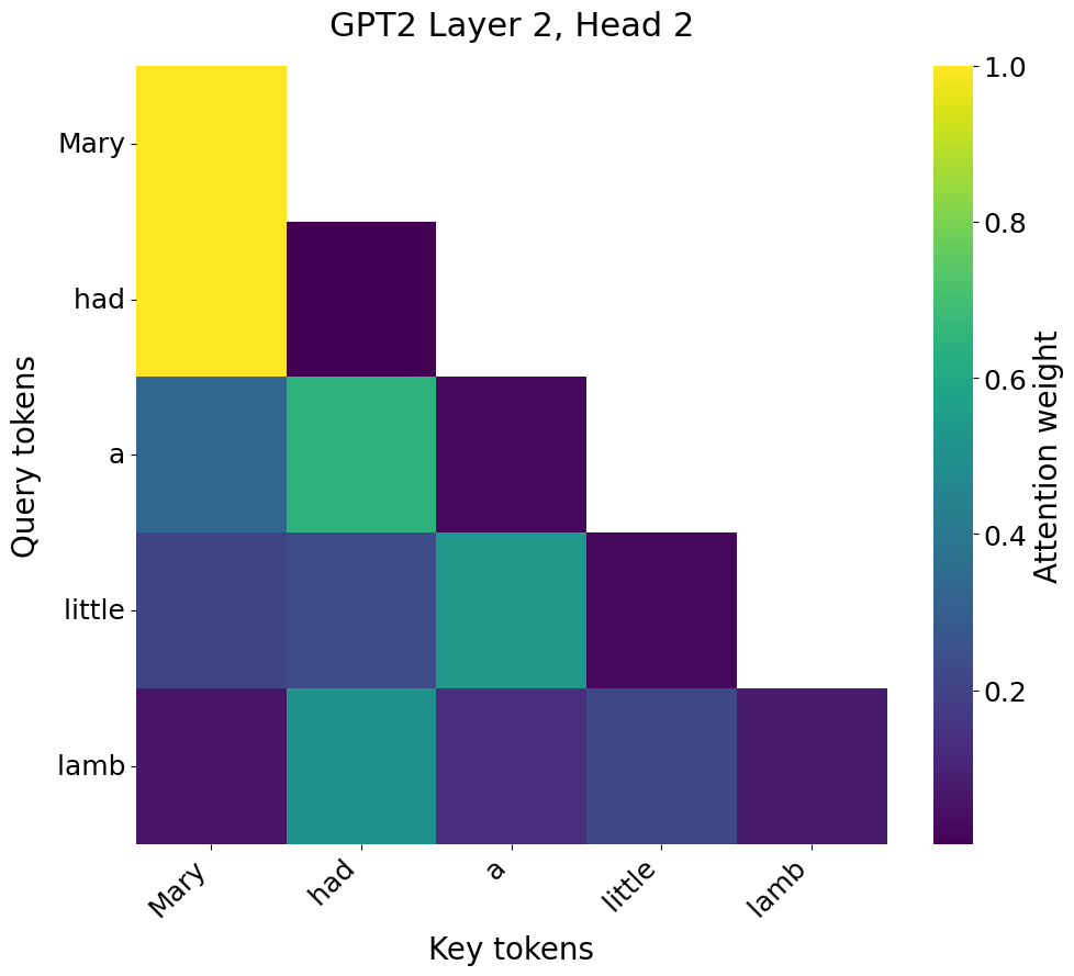What this means is that different inputs get potentially different attention patterns to operate linearly on them — "Mary had a little lamb" gets a (5, 5) attention pattern:

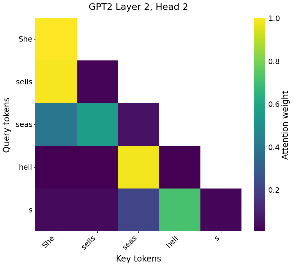
that is very likely different from the one "She sells seashells" gets:

while "Little Jack Horner sat in a corner" gets a bigger, potentially very different-looking attention pattern of its own:

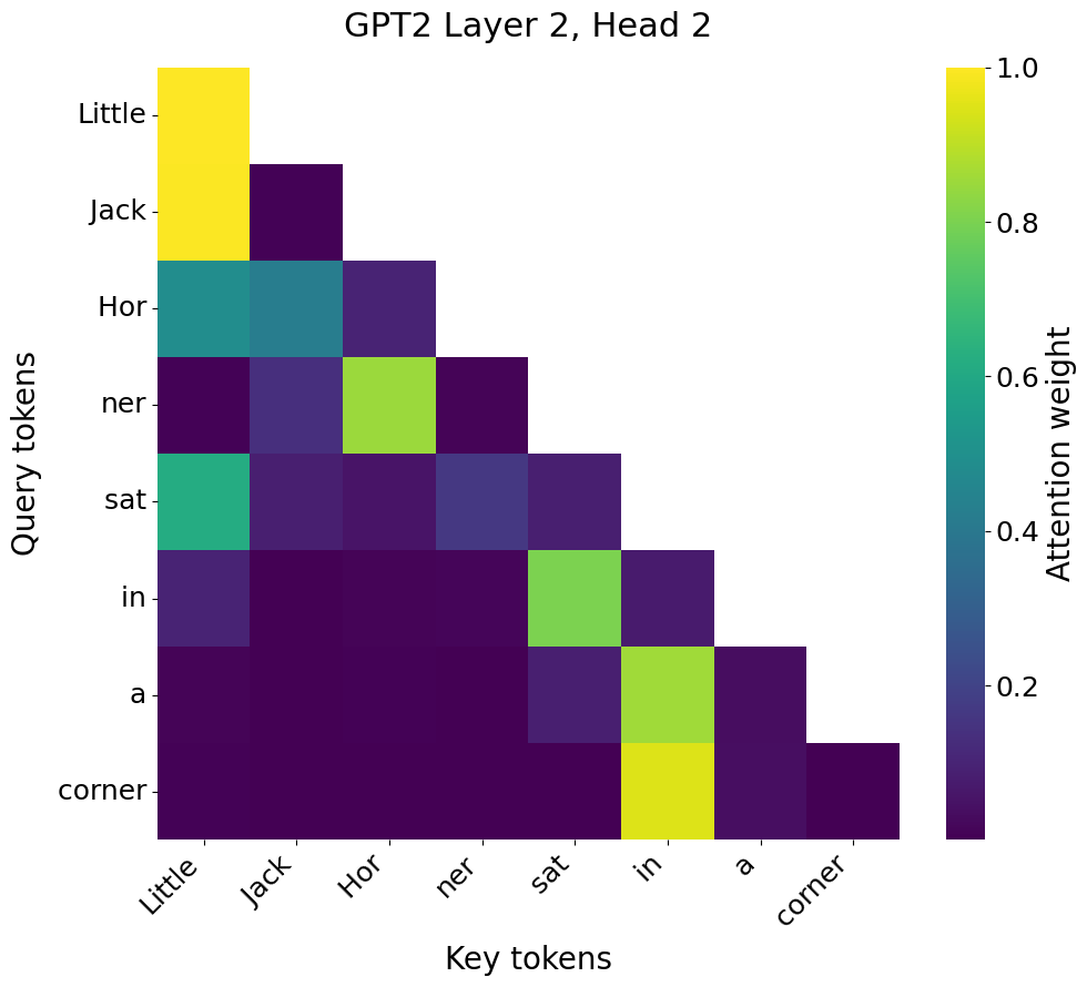
Compare this to a feedforward network or a CNN: the same layer/filter is applied to every input, no matter differences between inputs (I rush to add that this is by design and part of those architectures’ inductive biases).

Maybe part of the reason attention works so well is the data-dependence of its core transformation, which perhaps gives it uniquely expressive power? Maybe we’d like Hyena to have this property as well.

It turns out that the Hyena operator is data-dependent. The elementwise multiplications with projections of the input sequence inject data-dependence.

Let’s make this clearer by representing the Hyena operator as a product of matrices representing the convolution and elementwise multiplication operations. When we write a Hyena operator in this way, we will be able to show exactly which of its decomposing matrices are data-dependent.

Starting with the bare basics: how do we show elementwise multiplication and convolution as matrices at all?

Elementwise multiplication of two vectors is equivalent to multiplying one with a diagonal matrix:

Notice the output of the matrix multiplication above is exactly what we want: $v$ and $x$, multiplied elementwise.

Convolutions can be represented using something called Toeplitz matrices. For example, a short centered convolutional filter $k$ sliding over a sequence $x$ is equivalent to the matrix multiplication below:

Notice how the matrix structure captures the sliding window nature of convolution: each row represents the filter being shifted by one position.

Non-centered convolutions look different (the origin is at the filter’s edge):

Finally, let’s figure out the Toeplitz matrices of non-centered long convolutions (these are the kind of convolutions Hyena has). Imagine a fiter $[h_1, h_2, \dots, h_L]$ being slid over a sequence $[x_1, x_2, \dots, x_L]$. The filter is flipped over ($[h_L, h_{L-1}, \dots, h_1]$) and slid over the sequence. The Toeplitz matrix multiplication form is

Notice that both elementwise multiplication and convolution operations preserve causality, which is important for autoregressive language modeling. In both a diagonal matrix (elementwise multiplication) and a Toeplitz matrix (convolution), the upper triangular region is all zeros. This indicates that no position $i$ of the output is influenced by an input value that’s to the right of the $i$. In the output of a convolution, $y_1 = h_1x_1$ is influenced only by $x_1$, $y_2 = h_1x_2 + h_2x_1$ is influenced only by $x_1$ and $x_2$, and so on. It should be even easier to see that elementwise multiplication preserves causality: $y_1 = v_1x_1$ of the output of an elementwise multiplication is influenced only by $x_1$, $y_2 = v_2x_2$ is influenced only by $x_2$, and so on.

The figure below shows how Hyena implicitly creates a (seq_len, seq_len) matrix just like attention does. (I say implicitly because $\mathcal{O}(\mathrm{L^2})$ memory-consuming (seq_len, seq_len) Toeplitz matrices are never materialized in the GPU, thanks to FFT magic.) The (seq_len, seq_len) Hyena operator is a composition of matrices representing successive convolutions and elementwise multiplications:

The figure below makes it clearer where the data-dependency in the Hyena operator comes from: dense networks create projections of the input sequence that are used for elementwise multiplication, while convolutional filters are defined independently of the input sequence.

Hyena has sublinear parameter scaling and unrestricted context

The Hyena operator described so far has a critical shortcoming: the parameter count grows linearly with the input sequence length. Specifically, we need to store $N$ filters in memory that are each as long as the input sequence. But this means they need to be pretty darn long if we want to process long inputs. And it is in cases of very long context that we even want a subquadratic operator like Hyena; for shorter contexts, attention’s quadratic complexity isn’t as ugly.

Many other deep learning methods you can think of don’t have this problem. For example, a CNN made of the same (short) filter sizes, layer depths, etc, can be applied to images small and large. Even attention relies on fixed (d_model, d_head) matrices W_Q and W_K to generate the projections that in turn give us an attention matrix which can grow with the input.

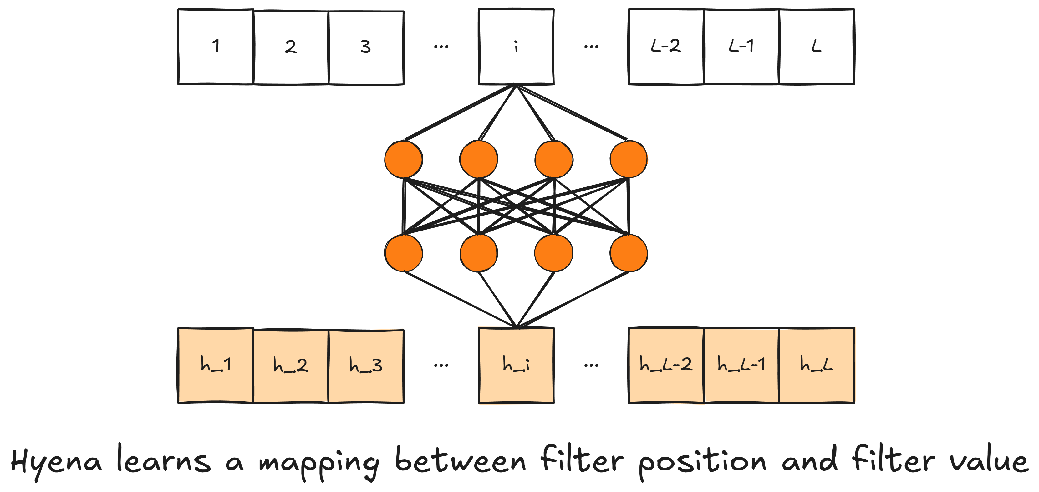
As it turns out, Hyena elegantly avoids a hard context length restriction by implicitly parametrizing its filters. Instead of storing filters directly in memory, a feedforward network learns a mapping between filter positions and filter values. For example, if you want a filter of length $10$, simply feed the numbers $1, 2, \dots, 10$ to a feedforward network. The networks maps $1$ to $h_1$ (the first filter value), $2$ to $h_2$ (the second filter value), and so on up to mapping $10$ to $h_{10}$. This network can generate a filter of any length on the fly! No need to cram long filters into memory. (Note that you don’t need to literally feed the positions one by one to the network; the filter values can be generated in parallel since they don’t depend on each other.)

This approach gives Hyena both sublinear parameter scaling (since the network generating the filters has a fixed parameter count) and unrestricted context length (since longer sequences just mean generating longer filters and input projections from those same fixed-parameter layers).

Hyena filters have an inductive bias of locality

After a filter is generated, it’s multiplied elementwise with an exponentially decaying function (specifically $\exp (-\alpha t)$). This exponentially decaying function is called the window function. This gives Hyena a “soft” locality bias: since earlier values of $h$ tend to be larger, tokens that are close by get more “attention”. Consider an arbitrary position in the output $i$. It’s $h_1x_i + h_2x_{i-1} + \cdots$. Since $h_1$, $h_2$ and other early filter values tend to be larger than later values like $h_{i-1}$ and $h_i$, close-by tokens like $x_i$ and $x_{i-1}$ get multiplied by relatively larger weights and therefore “get more attention”.

This figure from the paper makes the effect clear (notice how later values in $\mathrm{Window \circ FFN(t)}$ tend to be smaller):

Note this is a crucial architectural difference compared to vanilla attention! In standard attention, pairwise weights between even distant tokens can be arbitrarily strong; there’s no exponentially decaying window function to push these weights closer to zero. The use of an exponential decay to impose a locality bias was vindicated in an ablation in an earlier paper.

Empirical results

So, how well does Hyena do in practice?

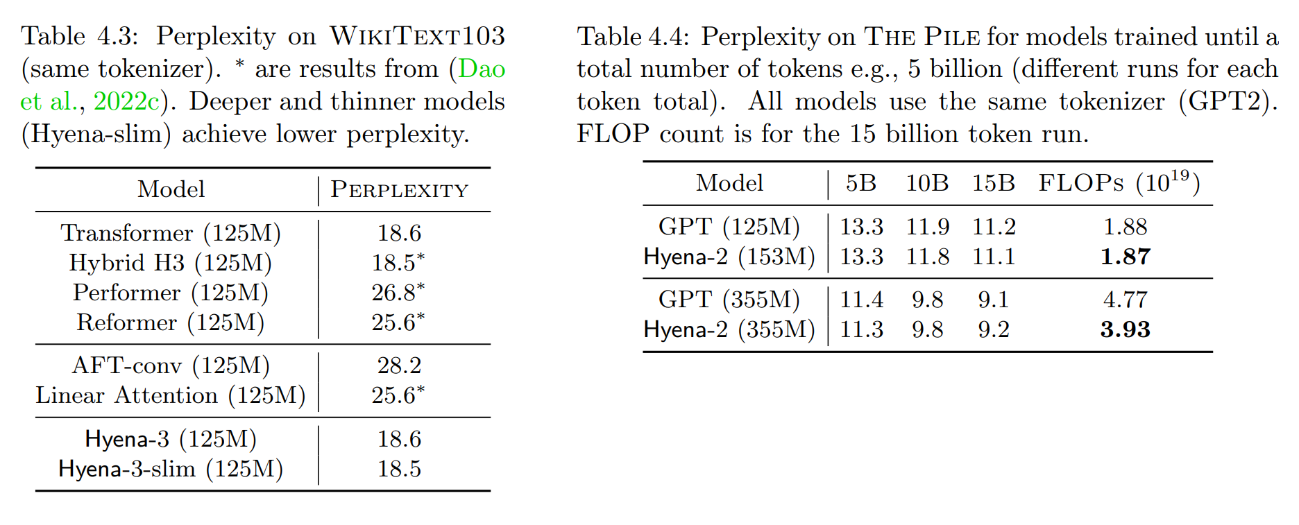
Quite well, as it turns out: it achieves about the same perplexity (a measure of the model’s accuracy on missing/next-token prediction; lower perplexity is better) as the transformer on the datasets WikiText103 and The Pile:

On downstream tasks like the Winograd schema challenge (answering questions of the form “The city councilmen refused the demonstrators a permit because they [feared/advocated] violence.” where mere grammatical reasoning is insufficient and something approaching world modeling is necessary), inferring a word’s intended meaning from its context, and reading comprehension, Hyena has comparable few-shot performance to a similarly-sized transformer, GPTNeo:

Though Hyena’s zero-shot performance on downstream tasks is more muted:

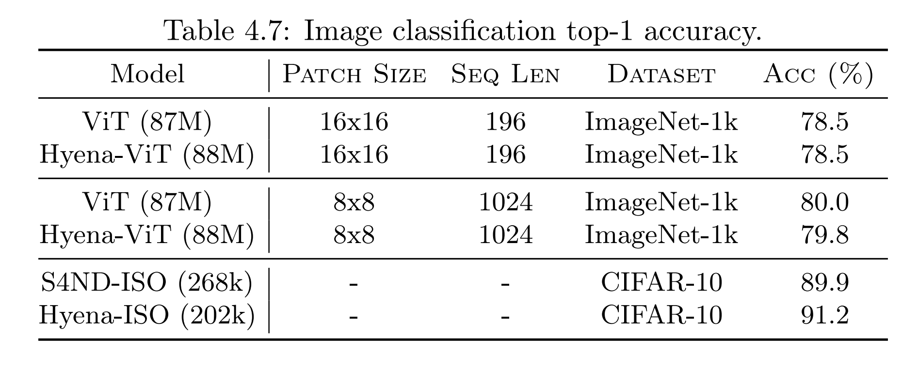
Finally, there’s some indication that Hyena is a good general deep learning operator. The authors drop-in replace attention layers in a vision transformer (ViT) with Hyena layers, and get comparable accuracy to the original ViT:

Conclusion

Hyena can be boiled down to: convolve text using fast Fourier transforms, and use elementwise multiplication to cheaply inject data dependency. Oh also, instead of storing long filters in memory, implicitly parametrize them using feedforward networks: sublinear parameter scaling and unrestricted context are nice.

Here a few of the most notable things from the paper I’ve left out in this post:

• Some architectural details, like depthwise short convolutions on input projections (for a kind of “denoising” effect along the embedding dimension), and sinusoidal activation functions for the networks parametrizing filters.
• Experiments on in-context learning at scale.
• Experiments on the best way to parametrize filters.
• Discussion about how Hyena is a generalization of other subquadratic operators like gated state spaces and Hungry Hungry Hippos.

For those details, I encourage checking out the original Hyena paper. Also read the Evo paper to learn exactly how it folds Hyena into its architecture. HyenaDNA, a precursor to Evo, is also an interesting read. Finally, if you’re interested in the broader attention alternatives literature, Sasha Rush’s overview is great.