Diffusion in 200 lines of Python
Diffusion underlies cutting-edge image, video and biological structure generation models, and some impressively fast text generation models. However, it has a reputation for being hard to learn. Part of the reason, I think, is that generative models like Stable Diffusion have many moving parts besides diffusion: U-Nets interacting with CLIP embeddings via cross-attention, variational autoencoders (VAEs), etc. Yet, a functional diffusion implementation can be really lean. For example, here are MNIST images generated with a model trained using a single ~200-line Python file:
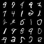
Pretty good! Most generations are actual digits. And the misses are close: the almost-7 at the top right and the mirrored 6 (fourth in the second row), for example.
In this post, I walk through the code for this. (You can play with it by cloning
this repo.) I intend this
to be a solid starting point for learning about diffusion. Only torch,
torchvision, and tqdm are dependencies. Simo
Ryu’s minimal diffusion
implementation is a strong
inspiration. I use ~high school algebra throughout. If you’re looking for a
math-free introduction, Sean
Goedecke’s is good.
Boilerplate
First, some imports:
import torch
import torch.nn as nn
import torch.nn.functional as F
from torch.utils.data import DataLoader
from torchvision import datasets, transforms
import torchvision.utils as vutils
import math
from tqdm import tqdm
import os
Next, device placement:
device = torch.device('cuda' if torch.cuda.is_available() else 'cpu')
Next, downloading and preparing the dataset:
# Data
transform = transforms.Compose([
    transforms.ToTensor(),
    transforms.Normalize((0.5,), (0.5,))
])
dataset = datasets.MNIST('./data', train=True, download=True, transform=transform)
dataloader = DataLoader(dataset, batch_size=batch_size, shuffle=True, num_workers=4)
Backbone model
At a high level, diffusion works by showing a neural network images with varying amounts of noise added to them, and training the network to predict the noise. During sampling, the network is shown pure Gaussian noise, its noise prediction is elicited and subtracted from the image, and the process is repeated until we’re left with a clean image. Of course, there’s no “correct” clean image recoverable from pure noise. As this Looking Glass Universe video puts it, we ask the model to effectively hallucinate a denoised image.
For the backbone model that learns to predict the noise in an image, the DDPM paper uses a U-Net with interspersed self-attention blocks. This is overkill for MNIST. A bog-standard convolutional neural network (CNN) with sinusoidal encodings to inject time information will work just fine.
While you’re probably familiar with CNNs as a bread-and-butter deep learning architecture, maybe you’re not so read up on sinusoidal position encodings. At least I wasn’t before implementing DDPM, because sinusoidal position embeddings have been obsolesced in language modeling by learned position embeddings and RoPE variants. If that’s the case, I encourage checking out Amirhossein Kazemnejad’s post. Not only are sinusoidal embeddings instrumentally useful to know about, as they’re alive and kicking in cutting-edge diffusion architectures like Stable Diffusion 3, they’re also one of the prettier ideas in deep learning.
Below is our backbone ~3.3-million parameter CNN. It has nine convolutional blocks. Each block is two convolutional layers, with group normalization and a nonlinearity (ReLU for simplicity) applied after each layer. The timestep embedding is calculated by applying a learned linear transformation to a sinusoidal encoding and added between the layers.
class SinusoidalPositionEmbeddings(nn.Module):
    def __init__(self, dim):
        super().__init__()
        self.dim = dim

    def forward(self, time):
        half_dim = self.dim // 2
        embeddings = math.log(10000) / (half_dim - 1)
        embeddings = torch.exp(torch.arange(half_dim, device=device) * -embeddings)
        embeddings = time[:, None] * embeddings[None, :]
        embeddings = torch.cat((embeddings.sin(), embeddings.cos()), dim=-1)
        return embeddings

class ConvBlock(nn.Module):
    def __init__(self, in_ch, out_ch, time_emb_dim):
        super().__init__()
        self.conv1 = nn.Conv2d(in_ch, out_ch, 3, padding=1)
        self.conv2 = nn.Conv2d(out_ch, out_ch, 3, padding=1)
        self.time_mlp = nn.Linear(time_emb_dim, out_ch)
        self.norm1 = nn.GroupNorm(8, out_ch)
        self.norm2 = nn.GroupNorm(8, out_ch)

    def forward(self, x, t):
        h = self.conv1(x)
        h = self.norm1(h)
        h = F.relu(h)

        time_emb = self.time_mlp(t)
        time_emb = time_emb[:, :, None, None]
        h = h + time_emb

        h = self.conv2(h)
        h = self.norm2(h)
        h = F.relu(h)
        return h

class ConvNet(nn.Module):
    def __init__(self):
        super().__init__()
        time_dim = 256
        self.time_mlp = nn.Sequential(
            SinusoidalPositionEmbeddings(time_dim),
            nn.Linear(time_dim, time_dim),
            nn.ReLU()
        )

        # Encoder
        self.enc1 = ConvBlock(1, 32, time_dim)
        self.enc2 = ConvBlock(32, 64, time_dim)
        self.enc3 = ConvBlock(64, 128, time_dim)
        self.enc4 = ConvBlock(128, 256, time_dim)

        # Bottleneck
        self.bottleneck = ConvBlock(256, 256, time_dim)

        # Decoder
        self.dec4 = ConvBlock(256, 128, time_dim)
        self.dec3 = ConvBlock(128, 64, time_dim)
        self.dec2 = ConvBlock(64, 32, time_dim)
        self.dec1 = ConvBlock(32, 32, time_dim)

        self.final = nn.Conv2d(32, 1, 1)

    def forward(self, x, t):
        t = self.time_mlp(t)

        # Encoder
        x = self.enc1(x, t)
        x = self.enc2(x, t)
        x = self.enc3(x, t)
        x = self.enc4(x, t)

        # Bottleneck
        x = self.bottleneck(x, t)

        # Decoder
        x = self.dec4(x, t)
        x = self.dec3(x, t)
        x = self.dec2(x, t)
        x = self.dec1(x, t)

        return self.final(x)
Training
Our main training function train() first instantiates the CNN and
AdamW as the optimizer. For each image x
in the MNIST dataset, we create a noisy variant x_noisy (I explain how
x_noisy is created later). The amount of noise added noise is controlled by
a timestep parameter t that goes up to 1000 (higher t = noisier image).
The model is fed x_noisy and t (the timestep helps the model gauge the
degree of noise that was added). Its output predicted_noise is compared
against noise using mean-squared
error loss, and the weights
are updated with backpropagation.
The function calc_x_t() generates x_noisy given x and t. At each
timestep, we add Gaussian noise $\epsilon$ scaled by some constant $k$ which is
generally less than 1:
Except that instead of a constant $k$, we use a noise schedule: a different scaling factor $k_t$ at each timestep $t$. Specifically, we increase $k$ over time. The intuition is that at later timesteps, when the image is mostly noise, adding a larger-than-usual dollop of noise doesn’t hurt and helps ensure we reach pure Gaussian noise.
But if we kept adding noise, the variance would grow without bound. This is a problem because the neural network would need to learn to handle wildly different input scales at different timesteps — imagine training a network where at t=10, inputs are roughly in [-3, 3], at t=500, inputs are roughly in [-50, 50], and so on. To keep the variance constant across time, we scale down the $x_{t-1}$ term so that the variance contribution from it is reduced:
\[x_t = \sqrt{1 - \beta_t} \cdot x_{t-1} + \sqrt{\beta_t} \cdot \epsilon\]For the next step, let’s define $\alpha_t = 1 - \beta_t$. If you do the algebra,
it turns out that $x_t$ has a closed-form expression in terms of the clean image
$x_0$; you don’t need a for loop from 1 to $t$:
(The notation $\prod_{s=1}^t \alpha_s$ means the product $\alpha_1 \cdot \alpha_2 \cdot \ldots \cdot \alpha_t$.)
The function calc_x_t() below directly uses this closed-form expression to
calculate x_t given x_0 and t.
# Diffusion hyperparameters
T = 1000
beta_start = 1e-4
beta_end = 0.02

# Training hyperparameters
batch_size = 128
lr = 1e-3
epochs = 100

# Noise schedule
betas = torch.linspace(beta_start, beta_end, T).to(device)
alphas = 1 - betas
alphas_cumprod = torch.cumprod(alphas, dim=0)
sqrt_alphas_cumprod = torch.sqrt(alphas_cumprod)
sqrt_one_minus_alphas_cumprod = torch.sqrt(1 - alphas_cumprod)

def calc_x_t(x_0, t, noise=None):
    if noise is None:
        noise = torch.randn_like(x_0)
    sqrt_alphas_cumprod_t = sqrt_alphas_cumprod[t].reshape(-1, 1, 1, 1)
    sqrt_one_minus_alphas_cumprod_t = sqrt_one_minus_alphas_cumprod[t].reshape(-1, 1, 1, 1)
    return sqrt_alphas_cumprod_t * x_0 + sqrt_one_minus_alphas_cumprod_t * noise

def train():
    model = ConvNet().to(device)
    optimizer = torch.optim.AdamW(model.parameters(), lr=lr)

    os.makedirs('samples', exist_ok=True)
    os.makedirs('checkpoints', exist_ok=True)

    for epoch in range(epochs):
        pbar = tqdm(dataloader, desc=f'Epoch {epoch+1}/{epochs}')
        total_loss = 0

        for batch_idx, (x, _) in enumerate(pbar):
            x = x.to(device)
            optimizer.zero_grad()

            t = torch.randint(0, T, (x.shape[0],), device=device).long()
            noise = torch.randn_like(x)
            x_noisy = calc_x_t(x, t, noise)
            predicted_noise = model(x_noisy, t)

            loss = F.mse_loss(predicted_noise, noise)
            loss.backward()
            optimizer.step()

            total_loss += loss.item()
            pbar.set_postfix({'loss': total_loss / (batch_idx + 1)})

        # Checkpoint
        if epoch > 0: # remove previous checkpoint to save disk space
            prev_checkpoint = f'checkpoints/checkpoint_epoch_{epoch:03d}.pt'
            if os.path.exists(prev_checkpoint):
                os.remove(prev_checkpoint)
        torch.save({
            'epoch': epoch,
            'model_state_dict': model.state_dict(),
            'optimizer_state_dict': optimizer.state_dict(),
        }, f'checkpoints/checkpoint_epoch_{epoch+1:03d}.pt')
Sampling
After 100 epochs through the MNIST training split, the model gets pretty good at predicting the noise! We can now use the model to generate images that look like MNIST digits. Importantly, this will be unconditional generation. That is, we cannot control outputs in any meaningful sense, since the model’s squinting and hallucinating a digit from pure noise. This is opposed to conditioning the generation on some text like “An expressive oil painting of a basketball player dunking, depicted as an explosion of a nebula.”, or some image-text pair like “Generate a Studio Ghibli version of this picture of my wife and me”. We usually condition image generation models via cross-attention with CLIP embeddings, but I’ve kept the details out of this post’s scope.
Our sampling function below, sample(), instantiates x as pure noise and
iteratively replaces it with a slightly denoised version generated by
calc_x_t_minus_one(). calc_x_t_minus_one() uses the trained model to predict
the noise in an image x_t given t. After T iterations/timesteps,
sample() returns the fully denoised x, which should look like a clean
digit.
The DDPM paper works out the following closed-form expression for $x_{t-1}$ given $x_t$ and $t$:
\[x_{t-1} = \frac{1}{\sqrt{\alpha_t}} \left( x_t - \frac{\beta_t}{\sqrt{1 - \prod_{s=1}^t \alpha_s}} \epsilon_\theta(x_t, t) \right) + \sqrt{ \frac{\beta_t(1 - \prod_{s=1}^{t-1} \alpha_s)} {1 - \prod_{s=1}^{t} \alpha_s} } \mathcal{N}(0, 1)\]($\epsilon_\theta(x_t, t)$ is the trained model’s prediction for the noise $\epsilon$ given $x_t$ and $t$. $\mathcal{N}(0, 1)$ is pure Gaussian noise.)
It is this closed-form expression that calc_x_t_minus_one() calculates.
Notice that the second term adds some noise to each denoised intermediate image $x_{t-1}$. This might seem strange: wouldn’t adding noise to a denoised image hurt? The intuition is that during the forward process, some noise is supposed to have been added at each timestep, so there are multiple less-noisy images $x_{t-1}$ that could have led to the current noisy image. Instead of deterministically taking a step back to $x_{t-1}$ using just the first term, we add a noise term to be able to sample from this diversity of valid paths. However, we omit the noise term for the final generation. Otherwise, we’d be unnecessarily blurring our outputs.
# Noise schedule
alphas_cumprod_prev = torch.cat([torch.ones(1).to(device), alphas_cumprod[:-1]])
sqrt_recip_alphas = torch.sqrt(1.0 / alphas)
posterior_variance = betas * (1 - alphas_cumprod_prev) / (1 - alphas_cumprod)

def calc_x_t_minus_one(model, x_t, t, t_index):
    betas_t = betas[t].reshape(-1, 1, 1, 1)
    sqrt_one_minus_alphas_cumprod_t = sqrt_one_minus_alphas_cumprod[t].reshape(-1, 1, 1, 1)
    sqrt_recip_alphas_t = sqrt_recip_alphas[t].reshape(-1, 1, 1, 1)

    model_mean = sqrt_recip_alphas_t * (x_t - betas_t * model(x_t, t) / sqrt_one_minus_alphas_cumprod_t)

    if t_index == 0:
        return model_mean
    else:
        posterior_variance_t = posterior_variance[t].reshape(-1, 1, 1, 1)
        noise = torch.randn_like(x_t)
        return model_mean + torch.sqrt(posterior_variance_t) * noise

@torch.no_grad()
def sample(model, n_samples=25):
    model.eval()
    x = torch.randn(n_samples, 1, 28, 28).to(device)

    for i in tqdm(reversed(range(T)), desc='Sampling', leave=False):
        t = torch.full((n_samples,), i, device=device, dtype=torch.long)
        x = calc_x_t_minus_one(model, x, t, i)

    model.train()
    return x
I added a sample() call at the end of each epoch in train():
        # Sample and save
        samples = sample(model)
        samples = (samples + 1) / 2  # Denormalize
        samples = samples.clamp(0, 1)

        grid = vutils.make_grid(samples, nrow=5, padding=2, normalize=False)
        vutils.save_image(grid, f'samples/epoch_{epoch+1:03d}.png')
Here are samples generated at epochs 1, 33, 67 and 100:
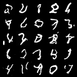
At epoch 1, we get mostly pure black or white. At epochs 33 and 67, we start to see vaguely digit-like shapes. And finally, at epoch 100, most shapes can be read off as actual digits.
Changing the backbone model
That wraps up our minimal DDPM implementation. This section is experimentation with the backbone model for fun.
I used a CNN because of its vision-specific inductive biases: local features like edges and color splotches, and translational equivariance. But any neural network that maps digit-shaped tensors (noisy images) to digit-shaped tensors (noise predictions) would work in principle. What happens if we swap out the CNN with a ~1.5-million parameter MLP?
class SmolMLP(nn.Module):
    def __init__(self):
        super().__init__()
        time_dim = 256
        self.time_mlp = nn.Sequential(
            SinusoidalPositionEmbeddings(time_dim),
            nn.Linear(time_dim, time_dim),
            nn.ReLU()
        )

        # MLP layers
        self.fc1 = nn.Linear(28*28 + time_dim, 512)
        self.fc2 = nn.Linear(512, 512)
        self.fc3 = nn.Linear(512, 512)
        self.fc4 = nn.Linear(512, 28*28)

    def forward(self, x, t):
        batch_size = x.shape[0]
        t = self.time_mlp(t)

        # Flatten image and concatenate with time embedding
        x_flat = x.view(batch_size, -1)
        x = torch.cat([x_flat, t], dim=1)

        # MLP layers
        x = F.relu(self.fc1(x))
        x = F.relu(self.fc2(x))
        x = F.relu(self.fc3(x))
        x = self.fc4(x)

        # Reshape back to image
        return x.view(batch_size, 1, 28, 28)
Since this MLP is a drop-in replacement for the CNN, using it is as simple as
going to train() and changing model = ConvNet().to(device) to model =
SmolMLP().to(device).
Here is the output using the MLP after 100 epochs:
It’s pure noise! Well, not pure: validation loss drops for ~5 epochs, but then it plateaus. >10x-ing model capacity by using a ~20.6 million-parameter MLP doesn’t help either:
class ChunkyMLP(nn.Module):
    def __init__(self):
        super().__init__()
        time_dim = 256
        self.time_mlp = nn.Sequential(
            SinusoidalPositionEmbeddings(time_dim),
            nn.Linear(time_dim, time_dim),
            nn.ReLU()
        )

        # Much larger MLP layers
        self.fc1 = nn.Linear(28*28 + time_dim, 2048)
        self.fc2 = nn.Linear(2048, 2048)
        self.fc3 = nn.Linear(2048, 2048)
        self.fc4 = nn.Linear(2048, 2048)
        self.fc5 = nn.Linear(2048, 2048)
        self.fc6 = nn.Linear(2048, 28*28)

    def forward(self, x, t):
        batch_size = x.shape[0]
        t = self.time_mlp(t)

        # Flatten image and concatenate with time embedding
        x_flat = x.view(batch_size, -1)
        x = torch.cat([x_flat, t], dim=1)

        # MLP layers
        x = F.relu(self.fc1(x))
        x = F.relu(self.fc2(x))
        x = F.relu(self.fc3(x))
        x = F.relu(self.fc4(x))
        x = F.relu(self.fc5(x))
        x = self.fc6(x)

        # Reshape back to image
        return x.view(batch_size, 1, 28, 28)
Here is the output we get:
This MLP is >6x larger than the CNN, but still completely useless. Picking the right inductive bias really seems to matter! This is the sweet lesson of deep learning: scale yields reliable log-linear improvements, but better architectures shift the whole curve down.
![]() Plots from Jared Kaplan and coauthors’ “Scaling Laws for Neural Language
Models” showing that
transformers
are an instrinsically better architecture than
LSTMs for language
modeling.
Plots from Jared Kaplan and coauthors’ “Scaling Laws for Neural Language
Models” showing that
transformers
are an instrinsically better architecture than
LSTMs for language
modeling.