Why L1 regularization creates sparsity
It’s well known that L1 regularization, which adds the absolute value of the parameters to the loss function, pushes some parameters to exactly zero, creating what’s called “sparse” features. On the other hand, L2 regularization adds the squares of the parameters to the loss, shrinking them without necessarily going all the way to zero. This is useful when all the features could be relevant.
There is a neat visualization for why this happens, which argues that L1 norm creates diamond-shaped level sets while L2 norm creates circular level sets:
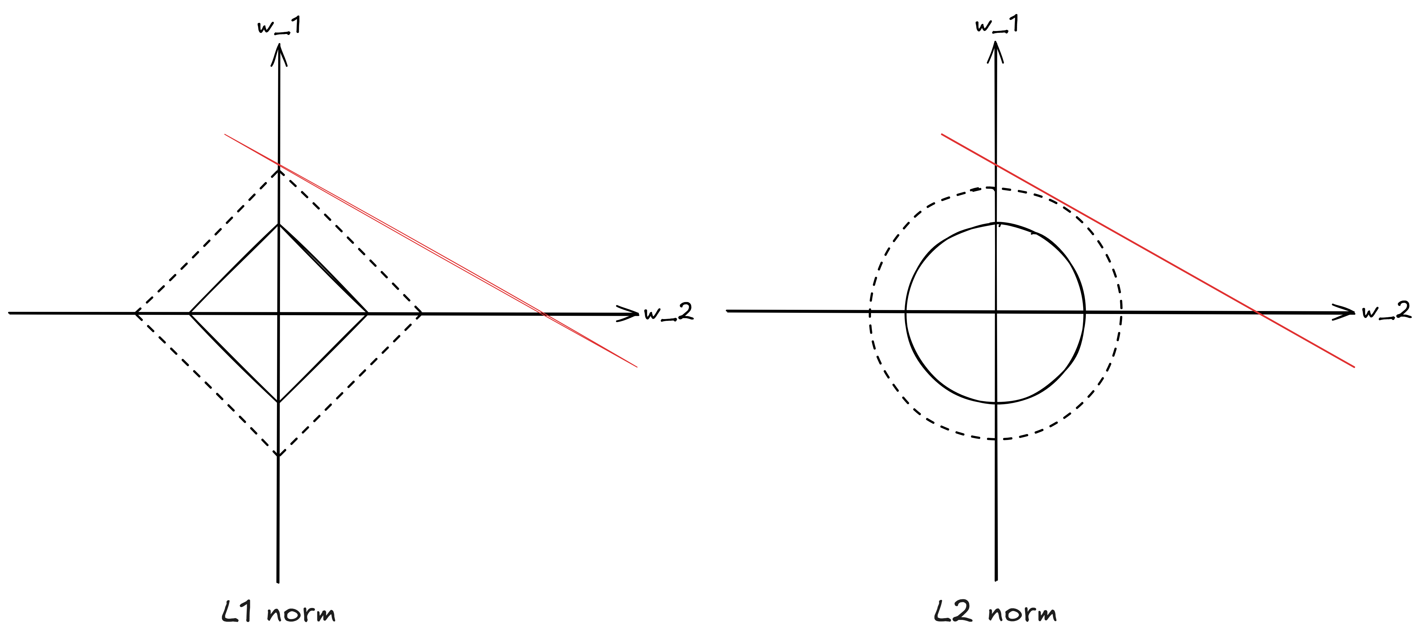 Adapted from Mxwsn’s
image on Wikipedia
Commons released under CC BY-SA
4.0.
Adapted from Mxwsn’s
image on Wikipedia
Commons released under CC BY-SA
4.0.
I think the visualization is solid, but here’s how I prefer thinking about L1 vs L2.
For a parameter w = 0.1:
- L1 penalty: |0.1| = 0.1
- L2 penalty: (0.1)2 = 0.01
For a parameter w = 0.01:
- L1 penalty: |0.01| = 0.01
- L2 penalty: (0.01)2 = 0.0001
Notice how L2’s quadratic nature means the penalty decreases much more rapidly as the parameter gets closer to zero, while L1 maintains a linear relationship. Looking at the gradients makes this even clearer (recall that you update the parameter proportionally to the gradient):
- For L1 regularization, the gradient of the penalty term is $\frac{\partial}{\partial w} \lambda |w| = \lambda \cdot \operatorname{sign} (w)$.
- For L2 regularization, the gradient is $\frac{\partial}{\partial w} \lambda w^2 = 2 \lambda w$.
This difference is crucial:
- L1’s gradient is always $\pm \lambda$ (except at w=0 where it’s undefined). This constant force pushes parameters toward zero with the same strength regardless of how close they are to zero.
- L2’s gradient is proportional to w. As parameters get closer to zero, the gradient also approaches zero, creating a progressively weaker push.
This maps perfectly to a physical analogy: L1 regularization is like a constant headwind, while L2 is like a spring. With L1, no matter how close you are to zero, the force pushing back remains the same. With L2, the closer you get to zero, the weaker the restoring force becomes (specifically, F=-kx in a spring according to Hooke’s law, which is linear with the displacement x similar to how the L2 gradient is linear with the parameter w).
This is why L2 can make parameters small but rarely exactly zero, while L1 is more likely to push parameters all the way to zero, making it useful for feature selection. Incidentally, this is also why lasso regression (L1 regularization) was backronymed as such — it lassoes the weights in towards zero.