Finding SAE features for concepts you choose
The mechanistic interpretability section of the paper “Genome modeling and design across all domains of life with Evo 2” (coauthored by the Goodfire team) contains a really clever way to label sparse autoencoder (SAE) features I haven’t seen elsewhere in the SAE literature. It deserves not being buried in a seventh of a supplementary figure, since it’s of broader interest to mech interp researchers outside biology. So, here’s a post explaining it.
Note that I assume familiarity with using SAEs to interpret large language models (LLMs). If you’re looking for an intro, Adam Karvonen’s post is excellent.
Concept-first rather than feature-first
The classic feature interpretation technique is automated interpretability (autointerp), introduced to the best of my knowledge in OpenAI’s “Language models can explain neurons in language models” and applied to SAE features in Anthropic’s “Towards Monosemanticity”. You show a language model like Claude or a GPT the highest activating tokens (with their surrounding context) on which a feature fires a lot, then ask the model what the feature is for. For example, if a feature consistently fires a lot on mentions of the Golden Gate Bridge, suspension bridges with “similar coloring” that are “often compared to the Golden Gate Bridge”, a paragraph in a story about driving to the Bridge, and so on, an LLM can tell it’s the Golden Gate Bridge feature. Browse through the highest activating tokens for Claude 3 Sonnet’s Richard Feynman, code error, self-improving AI, and exaggerated positive descriptions features for more examples. For rigor, of course, you’d want to evaluate the LLM-generated feature descriptions. You can do this in a bunch of ways, including the method described in the original OpenAI paper: simulate activations for a generated feature explanation using a different LLM instance, then score the overlap between the simulated and real activations.
But consider biology LLMs like Evo 2 and ESM 3 that are trained not on natural language, but on sequences of DNA, amino acids, etc. Autointerp does not work out of the box. An LLM cannot stare at a feature’s highest activating nucleotides or amino acids, and figure out what the feature means. Consummately experienced biologists cannot do this without supporting annotations.
While you can scaffold your feature-labeling LLM with UniProt and other annotations, InterPLM-style, you can also take a concept-first, rather than feature-first approach: look for biological concepts the model must have learned, just because they’re so fundamental to next nucleotide/amino acid prediction. For example:
- A DNA LLM should learn about coding sequences, i.e., regions of DNA that encode proteins. These have fundamentally different statistical properties from non-coding regions: they follow a triplet codon structure (every 3 bases encode an amino acid) creating regularities in the sequences, have higher GC-content, etc. Learning these statistical properties would probably make next-token prediction easier.
- A DNA LLM should learn about protein secondary structure (like alpha-helices and beta-sheets): DNA sequences encode proteins, and the functioning of these proteins depends enormously on their 3D structure. Evolutionary pressure maintains these patterns across genomes, and statistical correlations between DNA sequences and the resulting protein structures are strong enough to be captured during training.
- A DNA LLM should have a feature direction in its activation space for exon-intron boundaries. Exons are the coding regions that remain in the final messenger RNA and get translated into proteins, while introns are non-coding regions that get spliced out during mRNA processing. Boundaries between them have distinctive motifs (like the GU-AG rule at the 5’ and 3’ splice sites). Exons also generally have higher GC-content compared to introns. A DNA LLM needs to learn these patterns to effectively predict sequences across these transitions, similar to how natural language LLMs must learn sentence boundaries.
- A DNA LLM should learn about frameshift and premature stop codon mutations. Frameshift mutations occur when nucleotides are inserted or deleted in numbers that aren’t multiple of three, shifting the reading frame for all downstream codons. This creates a completely different set of amino acids being encoded after the mutation point, often introducing a premature stop codon (as the new, incorrect codon sequence is likely to eventually contain one of the three stop codons by chance). Premature stop codons halt protein synthesis early, resulting in truncated, almost always non-functional proteins. This creates strong selective pressure against such mutations in functional genes. A DNA LLM would notice that coding regions favor mutations that maintain reading frames and avoid premature stops.
So, we can start labeling SAE features by looking for these obviously useful features. But how exactly do we hunt for a feature for, say, coding regions? This is where the clever contrastive feature search algorithm comes in.
The contrastive feature search algorithm
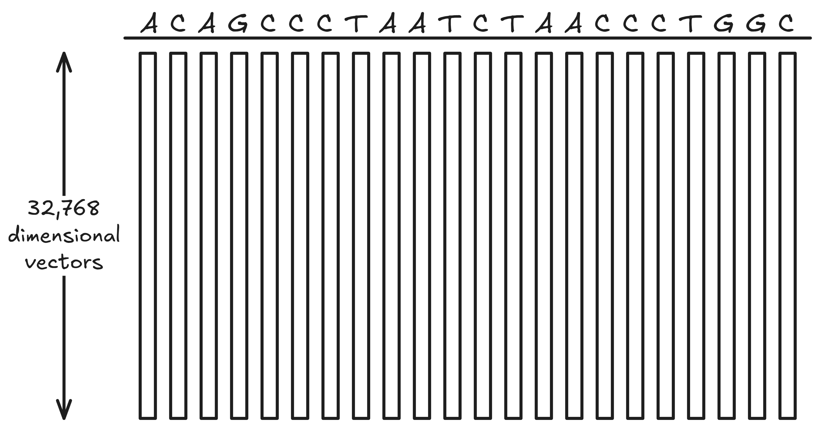
Say you want to find the SAE feature(s) for coding regions. You start by collecting all the 32,768-dimensional SAE vectors for a large chunk of DNA (say, 100,000 base pairs). That’s 100,000 32,768-dimensional SAE vectors.
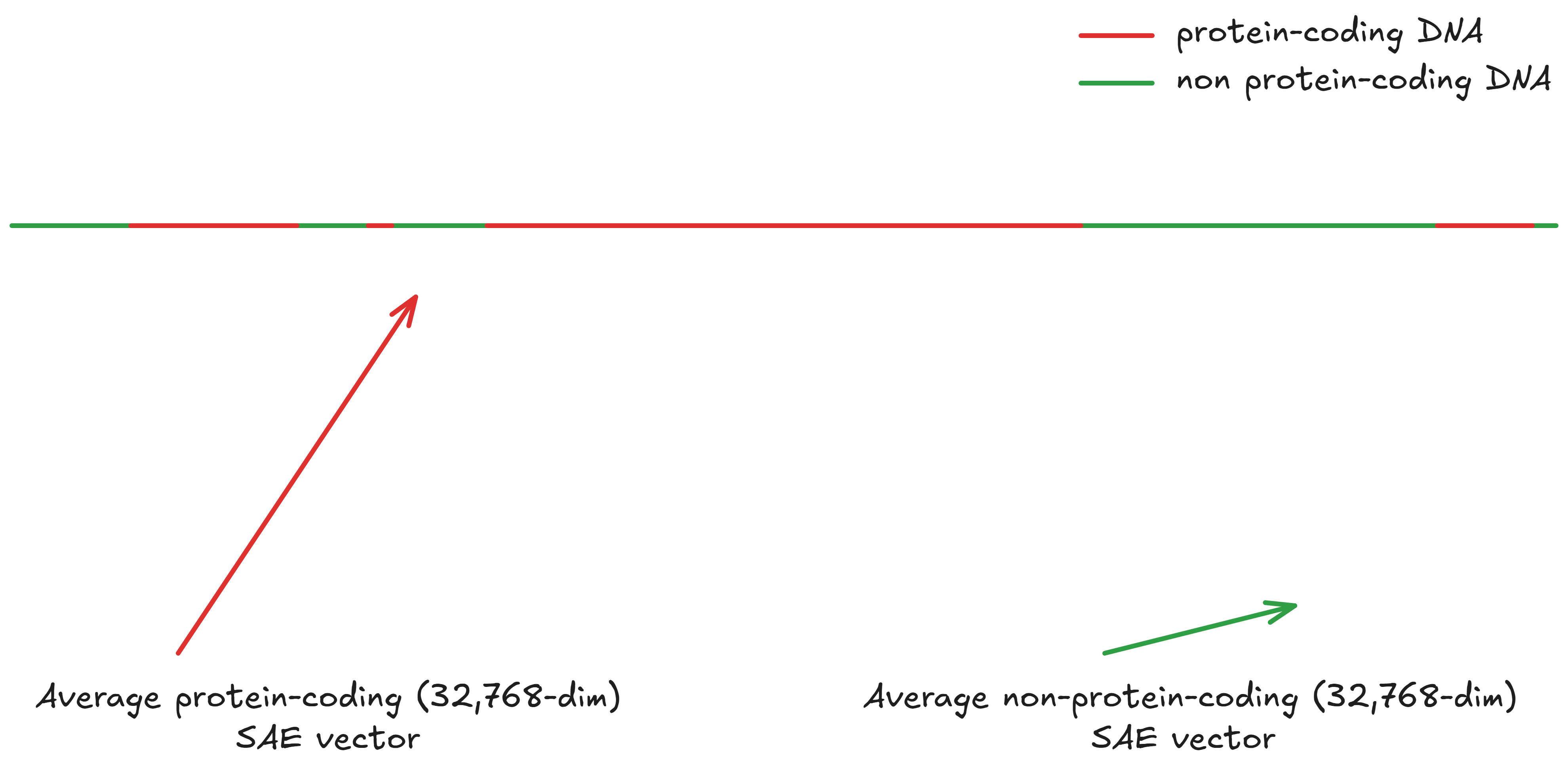
Next, you take the arithmetic mean of all the vectors for coding regions, and the mean of all the vectors for non-coding regions:
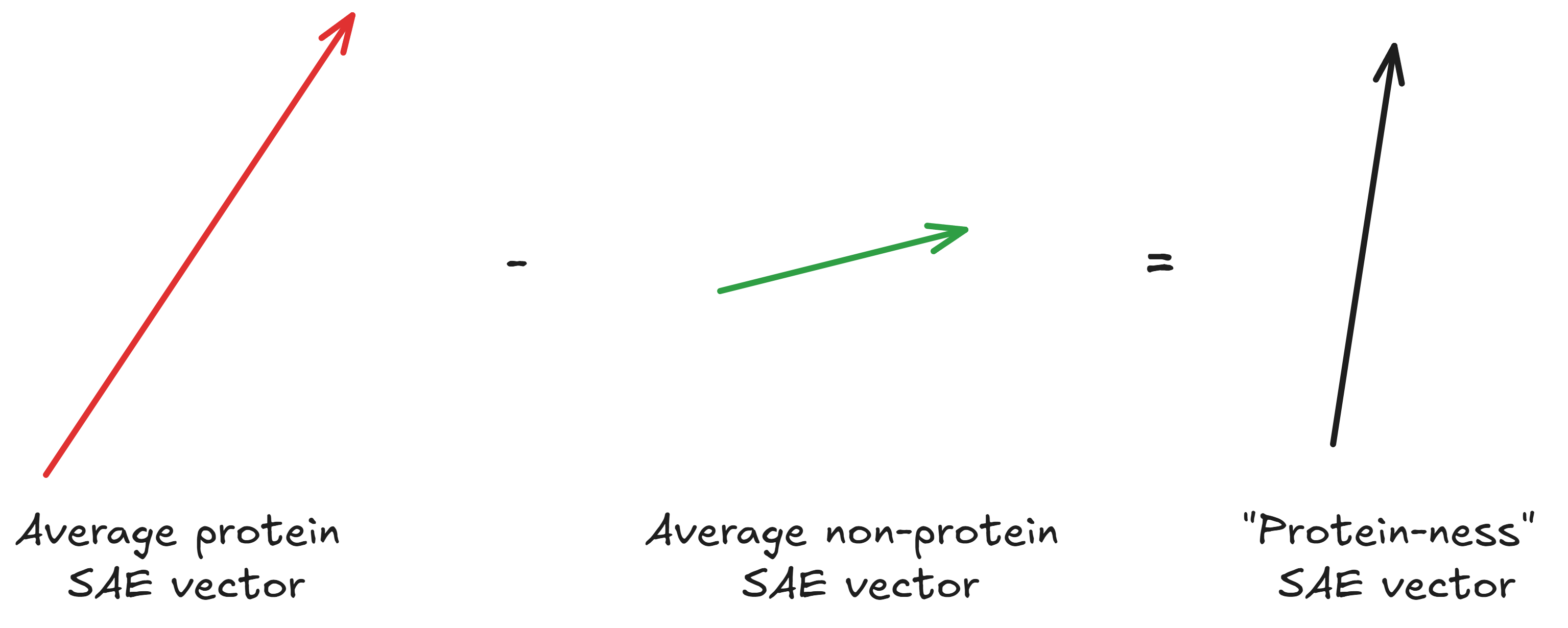
Then, you subtract the average non-coding SAE vector from the average coding SAE vector to get an SAE vector for “protein”-ness:
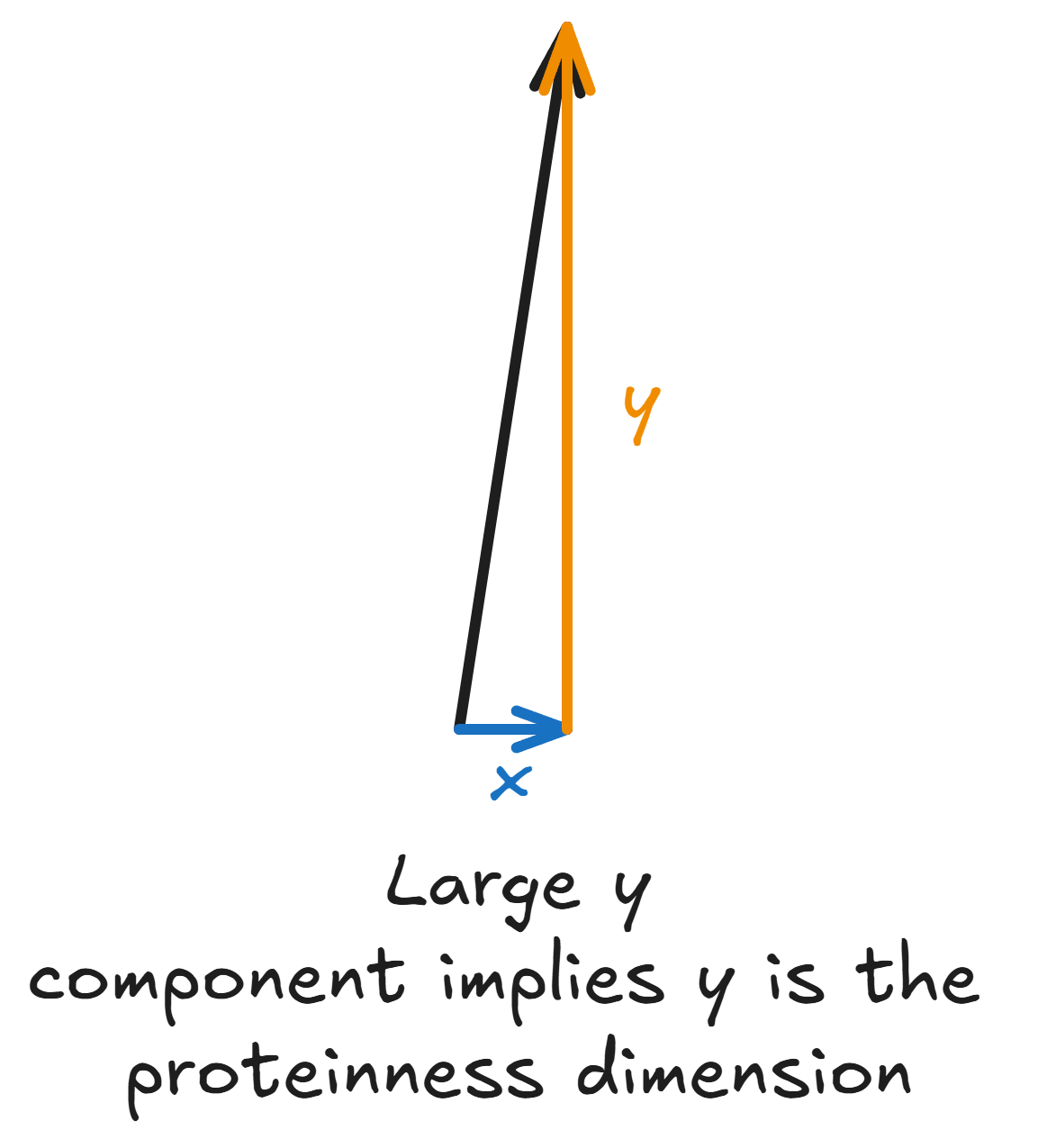
Now, recall that the protein-ness vector is still 32,768-dimensional. Presumably, not all of these dimensions are important: due to sparsity priors like L1 regularization or the BatchTopK activation function, our SAE uses only a few of these dimensions to encode information about any given concept (like protein-ness). So, as a denoising step, we select only the top 10 or so dimensions of the 32,768-dimensional protein-ness vectors, and call these 10 dimensions the “protein”-ness features. In the toy illustration, the protein-ness SAE vector has a tiny x-component and a large y-component. So, it’s the y direction that encodes protein-ness in our example.
Of course, we’d still like to stress-test our features against F1 scoring (and the Evo 2 authors do). But this is how the core algorithm of finding SAE features for concepts using contrastive search works.
An important subtlety: why do we care to subtract the non-protein vector at all? Why not just directly pick the top 10 features of the average protein-coding vector? Because the average protein SAE vector’s largest features may not be about protein-ness. The largest features could instead be bacterial-ness (if the chunk of DNA you picked was from E. coli, for example). Subtracting the non-protein vector is an important step in getting rid of these features you don’t care about.
Applications beyond biology
Contrastive feature search is a general algorithm for concept-first mech interp. Two applications stand out immediately:
- Interpreting sequence prediction models that are not trained on immediately-interpretable data (like natural language). For example, meteorological prediction models like Microsoft’s Aurora will be challenging to autointerp, but there are almost certainly motifs in atmospheric patterns that we can find SAE features for using contrastive search.
- Features for certain concepts in natural language models may be of special interest to us. For example, we might want to clamp down on/unlearn features for unsafe or buggy code, Islamophobia, racial slurs, etc. We might want to classify text that has a certain feature (say, use a spamminess SAE feature to filter email, as my friend Joe’s done). Contrastive feature search is a much quicker way to home in on these features than autointerp.